Robotics 101: Master the Fundamentals of Robot Design and Programming

Table of Contents

You've inherited a robotics project. The hardware sits in a corner. Someone on Slack is arguing about inverse kinematics. The simulation environment that was supposed to take two weeks is on month three. Procurement wants to know if you actually need the second LiDAR, and nobody on the team can answer because nobody agrees on what the robot is supposed to do yet.

The basics of robotics aren't a textbook chapter — they're the shared mental model that separates teams shipping skills in weeks from teams burning quarters on prototypes. This guide is for engineers, integrators, and technical leads who need conceptual fluency to make architecture, tooling, and deployment decisions — not to become control theorists by Friday.

By the end of it you'll be able to do seven things: identify your robot's archetype, explain the physics chain from kinematics through dynamics to control, choose between simulation and hardware deliberately, read a robot software stack diagram, set realistic latency budgets for your control loops, understand how modern training pipelines actually compress timelines, and pick a first concrete project that matches your team's constraints.

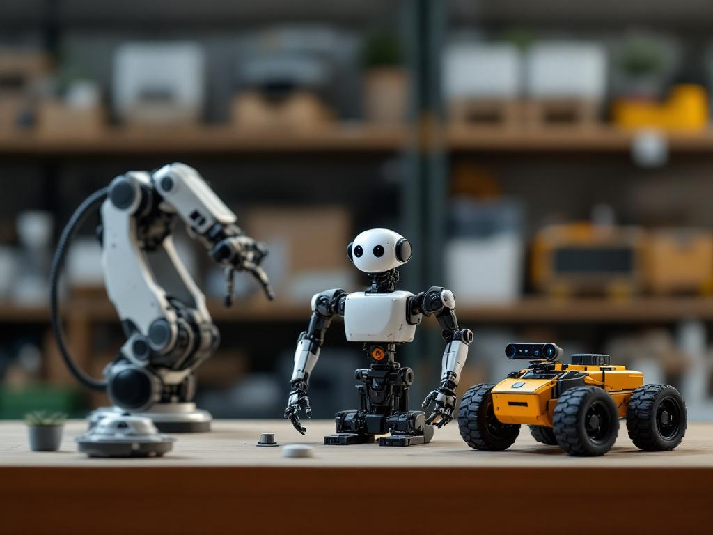
Table of Contents

• The Three Robot Archetypes: Why Architecture Decides Everything Downstream
• Kinematics, Dynamics, and Control: The Physics Chain You Can't Skip
• Simulation vs. Real Hardware: The Reality Gap and When to Cross It
• From Sensor to Servo: Reading a Robot Software Stack
• Real-Time Constraints: Why a Robot Can't "Think About It"
• How a Robot Skill Actually Gets Built Today
• Your First Robotics Project: A Week-One Checklist by Archetype
• FAQ — Quick Answers to the Three Questions Every Beginner Asks

---

The Three Robot Archetypes: Why Architecture Decides Everything Downstream

Most teams treat "robot" as a single category. It isn't. The hardware archetype you choose constrains your sensor stack, your control loop frequency, your simulation strategy, and whether pretrained policies even exist for your problem. Get this wrong at week one and every downstream decision — from procurement to staffing — bends around a bad assumption.

Three archetypes cover the vast majority of platforms a modern team will encounter.

Manipulators (fixed-base arms) typically have 6 or 7 degrees of freedom (DOF). The task space is a bounded reachable volume. Representative platforms include the Franka Research 3 (7-DOF, 855 mm reach), the Universal Robots UR5e (6-DOF, 850 mm reach), and the KUKA LBR iiwa. Inverse kinematics is the dominant computational problem. Sensors are often minimal: joint encoders, a wrist-mounted force/torque cell, sometimes a wrist camera. The design dimensions described by CMU Robotics Education — locomotion, end-effectors, purpose-alignment — collapse here to "no locomotion, end-effector is everything."

Mobile robots (wheeled or tracked) use differential drive, Ackermann steering, or omnidirectional wheels. The chassis itself has 2–3 DOF (x, y, heading). Examples: Clearpath Husky, warehouse AMRs, autonomous floor scrubbers. The dominant problem is SLAM (Simultaneous Localization and Mapping) and path planning. The sensor stack is heavier: 2D or 3D LiDAR, wheel odometry, IMU, often stereo cameras.

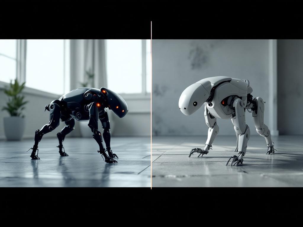
Legged and humanoid robots run from 12 DOF (most quadrupeds — Unitree Go2, Boston Dynamics Spot) up to 25–40+ DOF (Unitree H1, Figure 02, Tesla Optimus). The dynamics are inherently unstable; the robot is constantly falling and catching itself. This forces hard real-time control loops. The sensor stack adds joint torque sensing, foot contact sensors, and depth cameras to the IMU baseline.

Why does this matter for everything you do next? Manipulators have known, bolted-down base frames, so state estimation is trivial. Mobile robots must localize in a world that may change. Legged systems must do both — plus solve stability in milliseconds.

Dimension	Manipulator	Mobile Robot	Humanoid / Legged
Typical DOF	6–7	2–3 (chassis)	12–40+
Base	Fixed	Mobile, planar	Mobile, dynamic
Dominant problem	Inverse kinematics	SLAM + planning	Balance + locomotion
Control loop target	100–1000 Hz	10–100 Hz	500–1000 Hz
Primary sensors	Joint encoders, F/T, wrist cam	LiDAR, wheel odom, IMU	IMU, joint torque, depth
Sim-to-real difficulty	Moderate	Moderate	High

Control loop frequency targets come from physics, not preference. A balancing humanoid that updates torques at 10 Hz will fall before it can react; a manipulator placing a screw at 1000 Hz is wasting compute on a task that doesn't need it. The sensor differences cascade into the software stack. A manipulator team can ship without ever touching SLAM. A quadruped team cannot. A humanoid team without a real-time-capable kernel has chosen, whether they realize it or not, to fail.

Your robot's archetype — fixed base or mobile, six joints or forty — decides your control loop frequency, your sensor budget, and whether pretrained policies even exist for your problem. Pick wrong and every downstream choice gets harder.

The practical takeaway: before you spec hardware, write down which archetype you're building and which sub-problems that archetype forces on you. If you don't have an answer for "how does this robot know where it is?" within the first week, you have not yet chosen an archetype — you have only chosen a budget.

---

Kinematics, Dynamics, and Control: The Physics Chain You Can't Skip

Every robot, regardless of archetype, runs the same conceptual chain: geometry (kinematics) → forces (dynamics) → corrections (control). Read it from left to right and the rest of robotics stops looking like magic.

Kinematics: the geometry of motion

Kinematics describes where things are and how they move, ignoring why. Two problems live here.

Forward kinematics answers: given the joint angles, where is the end-effector? The textbook method is the Denavit-Hartenberg (DH) convention, which composes a chain of homogeneous transformation matrices — one per joint — and multiplies them to get the tool pose in the base frame. An open educational walkthrough on YouTube covers DH parameters, transformation chains, and Jacobians for engineers who want the mathematical detail.

Inverse kinematics (IK) answers the harder question: given a desired end-effector pose, what joint angles get me there? Hard because (a) it can have multiple valid solutions (elbow-up vs. elbow-down), (b) it can have no solution (the target is out of reach), and (c) it can hit singularities — configurations where the Jacobian loses rank and small Cartesian moves demand infinite joint velocity. The IK solvers you'll encounter in practice are KDL (the ROS default), TRAC-IK (better convergence on near-singular configs), and IKFast (analytical, compiled per robot).

Dynamics: how forces become motion

Dynamics is governed by the rigid-body equation:

M(q)q̈ + C(q,q̇)q̇ + g(q) = τ

Where M is the inertia matrix, C captures Coriolis and centripetal terms, g is gravity compensation, and τ is joint torque. You don't need to derive this. You need to know one thing: gravity compensation alone can consume 40–60% of motor torque on a horizontal arm. Ignoring dynamics is the reason naive position controllers oscillate, overshoot, and slam into hardstops.

Control: closing the loop

Control is the feedback loop that turns desired motion into motor commands. Four flavors dominate.

PID (proportional-integral-derivative) is still the workhorse of joint-level control. P reacts to current error, I eliminates steady-state offset, D damps oscillation. Tuning is empirical and is where junior engineers spend their first month.

Computed-torque (inverse dynamics) control uses the dynamics model as a feed-forward term, with PID correcting whatever the model gets wrong. Standard on every modern manipulator worth using.

Model Predictive Control (MPC) optimizes a control trajectory over a short future horizon, re-planning every cycle. It is the dominant approach for legged locomotion — the Boston Dynamics, Unitree, and MIT Cheetah lineages all use variants of MPC.

Learned policies (RL and imitation learning) replace or augment classical control with a neural network trained in simulation. The full pipeline appears later in this guide.

A worked example: manipulator reaches for a box on a conveyor

1. Vision system reports box pose in the camera frame.
2. Transform that pose into the robot base frame (forward kinematics of the camera mount).
3. Solve IK for a pre-grasp pose above the box.
4. Plan a collision-free trajectory through joint space.
5. Each control tick (1 ms): the dynamics model computes feed-forward torques, PID corrects residual error, motors execute.
6. The wrist force/torque sensor detects contact. The controller switches modes from position to impedance control.

Now contrast a quadruped trotting. The same chain runs, but the dynamics include unscheduled foot contacts, and the controller must replan footstep placement at 100+ Hz using MPC. The chain is identical; the difficulty of each link is not.

If your team can't draw this five-step loop on a whiteboard in 60 seconds, the team is not yet ready to argue about which IK solver to use.

---

Simulation vs. Real Hardware: The Reality Gap and When to Cross It

Simulation is cheap, parallel, safe, and fast. You can run 4,096 instances of a policy in NVIDIA Isaac Sim on a single GPU. Hardware is slow, dangerous, and serial — but it is the only place that tells you whether your robot actually works.

The reality gap is the systematic difference between simulation and the physical world that causes sim-trained policies to fail on deployment. Four sources contribute to it.

Contact dynamics. Rigid-body physics engines (PhysX, MuJoCo, Bullet) approximate friction and contact differently. A grasp that succeeds in sim can slip in reality because the friction coefficient or the compliance model was wrong by 15%.

Sensor noise. Simulated LiDAR is clean. Real LiDAR has dropouts, retroreflective glare, and multi-path artifacts on glossy floors. Simulated cameras have perfect color; real cameras have rolling shutter, auto-exposure lag, and IR contamination from sunlight.

Actuator dynamics. Real motors have backlash, friction, thermal drift, and current limits that physics engines either approximate poorly or ignore. A policy trained against ideal torque control will fight a real motor that takes 2 ms to ramp current.

Latency. Simulation is deterministic. Real systems have variable USB jitter, network latency, and OS scheduling hiccups. A 5 ms tail latency on a 1 kHz loop is a control failure.

Three tools narrow the gap.

Domain randomization trains the policy across thousands of randomized physics parameters (friction, mass, motor delay, camera FOV) so the policy learns a behavior that's robust to any plausible reality.

System identification measures the real robot's actual parameters — link masses, joint friction curves, motor response — and loads them into sim so the trained policy starts closer to truth.

Real-to-sim pipelines capture the deployment environment with LiDAR or photogrammetry and reconstruct it as a physics-ready sim asset. This is the direction NVIDIA Isaac, Genesis, and MuJoCo MJX are converging on, and it is the core of how full-stack robotics AI platforms collapse training timelines.

Factor	Simulation-First	Hardware-First
Cost per iteration	Near-zero (compute only)	High (wear, breakage, operator)
Iteration speed	100×–1000× real time	1× real time
Parallelism	Thousands of envs at once	One robot, one trial
Safety	Risk-free	Collisions, drops, falls
Best for	Locomotion, contact-rich manip, vision policies	Calibration, teleop data, last-mile tuning

When to start in simulation: contact-rich manipulation (peg insertion, deformable handling), legged locomotion (every team that ships a working walker trains in sim first), and vision-based policies where you can synthesize labeled data cheaply.

When to start on hardware: simple pick-and-place with well-modeled objects, teleoperated data collection for imitation learning, and sensor characterization and calibration.

The archetype heuristic is brutal but accurate. Humanoids: simulation is mandatory. Manipulators with contact: simulation-heavy with hardware fine-tuning at the end. Mobile robots in known maps: hardware-first is often the faster path. Modern GPU-parallel simulators exist precisely to push the threshold of "sim-first viable" outward — they don't make hardware optional.

Simulation trains your policy a thousand times faster than reality. Hardware tells you which of those thousand lessons were lies. Modern robotics teams ship by doing both deliberately, not by choosing one.

---

From Sensor to Servo: Reading a Robot Software Stack

Most teams treat the software stack as a black box labeled "ROS." It isn't one thing. Walk it top-down by layer, name the tools that live in each, and the architecture stops feeling like a folklore.

Layer 1 — Sensor drivers and acquisition

Raw data from LiDAR (Velodyne, Ouster, Livox), cameras (Intel RealSense, Stereolabs ZED), IMU, and joint encoders. Drivers publish standardized message types — sensor_msgs/PointCloud2, sensor_msgs/Image, sensor_msgs/Imu. The latency budget here is sub-millisecond for joint encoders and 10–50 ms for camera frames at 30 fps.

Layer 2 — Perception and state estimation

Point cloud filtering, object detection (YOLO, GroundingDINO), SLAM (Cartographer, RTAB-Map, ORB-SLAM3), sensor fusion (Extended Kalman Filters and factor graphs like GTSAM). This layer produces a structured world model from raw bytes. Get this wrong and every downstream layer is operating on hallucinations.

Layer 3 — Planning

Global path planners (A*, RRT, RRT*), local planners (DWA, TEB for mobile bases), and motion planners for arms (MoveIt 2, OMPL). Output is a trajectory — a sequence of waypoints in joint space or Cartesian space.

Layer 4 — Control

Trajectory tracking, joint-level PID, MPC, or a learned policy. Output is joint torques, velocities, or position commands.

Layer 5 — Hardware interface

ros2_control, EtherCAT, CAN bus, manufacturer SDKs (Franka FCI, UR RTDE, Unitree SDK). Pushes commands to motor drivers, reads back joint state.

The middleware that holds it together

ROS 2 (current LTS: Jazzy Jalisco) sits across all five layers. It provides DDS-based publish/subscribe, service calls, parameter management, and — critically — the standardized message contracts that let you swap a UR5e for a Franka without rewriting perception. Automate.org's industry overview covers the broader industrial context for why standardization matters at this layer.

Modern AI-first stacks insert a policy layer between planning and control: a neural network that takes perception output and emits action directly, sometimes replacing planning entirely. Open-source frameworks like cap-x, LeRobot, and Isaac Lab standardize how these policies are trained, packaged, and loaded onto edge inference hardware. A Jetson Orin Nano (40 TOPS class) handles most manipulation and mobile policies. A Jetson AGX Orin (275 TOPS class) handles humanoid-scale policies with vision in the loop.

Here's the practical insight that nobody explains until you're three months in: the reason a team can swap hardware vendors without a rewrite is that ROS 2 message contracts (sensor_msgs/PointCloud2, geometry_msgs/Twist, trajectory_msgs/JointTrajectory) are stable across vendors. The reason teams can't swap quickly is that the policy and the calibration are bound to the specific hardware kinematics. The interface is portable. The intelligence is not — unless you've structured it to be.

---

Real-Time Constraints: Why a Robot Can't "Think About It"

In robotics, late is wrong. A control command that arrives 5 ms after its deadline isn't slightly suboptimal — it's a failure mode. Three real-time categories exist, and they map directly to where your code runs.

• Hard real-time: Missing a deadline causes system failure. The robot falls, the cut goes through the wrong material, the gripper crushes the part. Required for legged balance, force-controlled assembly, and surgical robotics.
• Firm real-time: Missed deadlines produce useless output (drop the frame, skip the cycle) but don't cascade. Vision-based servoing typically lives here.
• Soft real-time: Missed deadlines degrade quality but the system recovers. High-level path planning, user interface updates, telemetry.

These map to robot archetypes with specific numbers.

• Humanoid balance and legged locomotion (hard, 1–2 ms): A 500–1000 Hz inner control loop. The Boston Dynamics Atlas, Unitree H1, and MIT Cheetah lineage all run their balance controllers in this band. Put it on a non-real-time OS and the robot falls during the first scheduler hiccup.
• Force-controlled manipulation (hard, 1–4 ms): Assembly, polishing, and contact-rich tasks need 250–1000 Hz force loops. The Franka Control Interface runs at 1 kHz specifically because anything slower destabilizes contact.
• Mobile robot obstacle avoidance (firm, 50–100 ms): A warehouse AMR at 2 m/s travels 10 cm in 50 ms. Reaction times above that produce collisions at scale; well below that is wasted compute.
• Task planning and re-planning (soft, 100–1000 ms): "Pick the next item from the bin" can take a quarter second without breaking anything. This is where Python, LLM-based planners, and cloud calls are safe to live.

The tooling implication is concrete. Low-level control runs in C++ on a real-time kernel — PREEMPT_RT Linux, Xenomai, or QNX. High-level reasoning runs in Python on a generic OS, often offloaded to a separate compute board. Edge inference boxes in the Jetson AGX Orin class can host both with proper CPU isolation and partitioning: isolate cores 0–3 for the real-time control loop, leave cores 4–11 for perception, ML, and ROS 2 nodes.

If your architecture diagram has a Python node in the 1 kHz path, you have a bug that will surface as a falling humanoid in three months. Move it now.

---

How a Robot Skill Actually Gets Built Today: Capture, Train, Package, Deploy

If your mental model for "training a robot" is hand-coded behavior trees, update it. The modern pipeline has four stages, and each one has collapsed dramatically in the last 24 months.

Step 1 — Environment capture

The training environment must match the deployment environment, or the reality gap eats you. Three approaches dominate.

Hand-built sim means an engineer models the workspace in URDF (for robots) and USD or SDF (for environments). Slow, generic, low fidelity. Useful for early algorithm bring-up, weak for deployment-grade policies.

Photogrammetry, NeRF, and Gaussian splat capture a real space with a phone or camera and reconstruct it as a mesh or radiance field. Good visual fidelity, weak physics — you get a pretty room but the friction and mass properties are guessed.

Real-to-sim LiDAR scanning captures both geometry and material properties and produces a physics-ready sim asset of the actual deployment environment. This is the direction NVIDIA Isaac, Genesis, and the OpenKinematics pipeline are pushing, because it shrinks the reality gap before training even starts.

Step 2 — Policy training

Two paradigms dominate, with a third increasingly stacking on top.

Reinforcement learning (RL) has the robot try actions in simulation, get rewards, update the policy. Standard for locomotion. PPO is the workhorse algorithm. GPU-parallel simulators (Isaac Lab, MuJoCo MJX) can run 4,096–16,384 environments simultaneously, collapsing what used to be a six-month training run into hours.

Imitation learning has the robot watch teleoperated demonstrations and learn to copy them. Dominant for manipulation. Diffusion policies and the Action Chunking Transformer (ACT) are the current state of the art.

Pretrained foundation policies — RT-2, Octo, Pi-0 — are generalist models you fine-tune on your specific task. This stack-on-top approach is what aggressively compresses the timeline. Instead of training from scratch, you start from a model that already knows what an arm and a gripper are and teach it your task with hundreds of demonstrations instead of tens of thousands.

Step 3 — Packaging

A trained policy is a set of weights plus a runtime contract: what observations it expects, what actions it outputs, what coordinate frames it assumes, what frequency it runs at. Packaging means wrapping all of this into a deployable artifact — typically a Docker container or a serialized model (ONNX, TorchScript, TensorRT) with a ROS 2 node wrapper.

This sounds boring. It is the single most underestimated source of project delay in robotics.

Step 4 — Deployment to edge

The packaged policy ships to onboard compute. Jetson Orin Nano (40 TOPS, ~$500 board) handles most manipulation and mobile robot policies. Jetson AGX Orin (275 TOPS) handles humanoid-scale policies with vision. The runtime loads weights, subscribes to sensor topics, publishes actions, and runs the policy at the required frequency — typically 10–100 Hz for learned policies, with classical control underneath at 1 kHz.

Why timelines have collapsed

The traditional pipeline — hire ML engineers, build sim from scratch, collect data, train for weeks, debug sim-to-real, integrate with ROS 2, build deployment runtime — is a 6–12 month effort for a first skill. The modern pipeline — capture the environment, fine-tune a pretrained policy, package, deploy — collapses to days for teams using cloud sim training and managed deployment platforms. Open-source frameworks like cap-x and full-stack platforms encode this pipeline so teams don't rebuild it each project.

Be honest about the limits. This works today for well-bounded skills: pick-and-place on known objects, navigation in scanned environments, locomotion gaits on supported quadrupeds. It does not yet work for fully general "do anything in the kitchen" tasks. The compression is real but not infinite, and any vendor claiming otherwise is selling you a demo, not a deployment.

Training a robot skill used to mean hiring a PhD and waiting two quarters. With pretrained policies, GPU-parallel simulation, and packaged edge runtimes, the same loop now closes in days. The bottleneck moved from algorithms to integration.

---

Your First Robotics Project: A Week-One Checklist by Archetype

You have the vocabulary. Now pick a track. The forcing question is: which archetype are you building, and what's your team's actual constraint — time, expertise, or hardware budget?

Track A — The Conceptual Foundations Path (you need to understand before you build)

1. Install ROS 2 Jazzy on Ubuntu 24.04, or pull the official Docker image. Verify with ros2 topic list on the talker/listener demo.
2. Run the TurtleBot3 simulation tutorial end-to-end — it covers navigation, SLAM, and the message-passing model in one workflow.
3. Work through the forward and inverse kinematics module of the open robotics course. Implement a 2-DOF arm IK solver in Python. Plot the workspace.
4. Read the MoveIt 2 "Getting Started" guide and run a pick-place example in RViz with a simulated Panda or UR5.
5. Measure: write down the control loop frequency, planning latency, and end-to-end action latency for your sim example. You now have a baseline that means something.

Track B — The Hardware-First Path (you have a robot on the bench)

1. Calibrate sensors first. Camera intrinsics with a checkerboard, LiDAR-to-base transform via a known fiducial, joint zero positions per the vendor procedure. Skipping this poisons everything downstream and you won't know why.
2. Get teleoperation working before autonomy. If you can't drive the robot manually through your task, no policy will either.
3. Collect 50–100 teleoperation demonstrations of your target task. This is your training data for imitation learning.
4. Deploy a pretrained foundation policy (Octo, Pi-0, or a platform-provided baseline) and fine-tune on your demos.
5. Measure task success rate across 20 trials. Iterate on data quality, not on hyperparameters.

Track C — The Platform Path (you need to ship, not learn)

1. Identify your target hardware (Franka, UR, Unitree, custom) and your target task with a concrete success metric.
2. Evaluate full-stack robotics AI platforms against your task and hardware compatibility. The set worth comparing today includes OpenKinematics alongside covariant.ai, intrinsic.ai, skild.ai, and physicalintelligence.company.
3. Capture your deployment environment — LiDAR scan or video walkthrough — as training input. The fidelity here determines how small your reality gap will be.
4. Use cloud simulation training to produce a policy, then deploy to edge hardware (Jetson-class) in a single packaging step.
5. Validate on real hardware against the same success metric you'd use in Track B. Iterate the environment capture, not the model internals.

The fastest path to a working robot is the one that matches your team's actual constraints — time, expertise, and hardware budget. Pick the track, do the five steps, then come back for the next layer.

---

FAQ — Quick Answers to the Three Questions Every Beginner Asks

• Do I need to learn ROS 2 before starting? Not before — but soon. You can run sim examples and even some pretrained policies without writing ROS code. The moment you integrate two components (a sensor and a controller, a planner and an arm), ROS 2's standardized message contracts save weeks of glue code. Recommended sequence: run examples first, learn the publish/subscribe model second, write your own nodes third. By the time you have a working prototype, you should be comfortable reading a launch file and debugging with ros2 topic echo.
• What programming language should I learn for robotics? Python for perception, planning, ML, and high-level logic. C++ for real-time control, drivers, and anything in a hard-real-time loop. Most modern robotics frameworks (ROS 2, MoveIt 2, Isaac Lab, cap-x) expose Python APIs that call into C++ underneath. Start in Python. Learn enough C++ to read driver code by month three. If you've only worked in MATLAB or Simulink, plan a deliberate transition window — the algorithms transfer, the deployment ecosystem does not.
• How long until I can deploy a trained skill on real hardware? In practice: with a pretrained policy and a packaged deployment platform, working pick-and-place on a known arm in days; locomotion on a supported quadruped in 1–2 weeks. Without pretrained policies and packaged tooling — building the sim, the training pipeline, and the deployment runtime from scratch — 3–6 months is realistic for a first skill, longer for the first team. The gap between those two timelines is the gap that real-to-sim pipelines and managed robotics AI platforms exist to close.