Mastering Robotic Control Systems: A Beginner's Guide to Motion Control

Your robot arm reaches the target — then overshoots by 4 degrees, settles, drifts back. Or your wheeled rover tracks straight on tile and curves on carpet. The motors are fine. The mechanical assembly is fine. What's broken is invisible: the loop between command and motion.

Robotic control is the discipline of closing that loop. It is what separates a machine that moves from a machine that moves predictably under load, voltage sag, friction shifts, and the dozen other disturbances that arrive uninvited the moment you take a project out of simulation. This guide takes you from open-loop guessing to closed-loop engineering — covering feedback architecture, PID logic, hardware selection, tuning methodology, advanced control patterns, and diagnostics.

It is written for hobbyists, students, and early-stage engineers crossing the gap between "robot that moves" and "robot that moves repeatably." If you have ever stared at a serial plot watching your setpoint and your actual position trace two completely different stories, this is for you.

Table of Contents

• Why Open-Loop Commands Fail the Moment Load or Friction Changes
• Position, Velocity, and Speed Feedback: Choosing the Right Sensor for the Task
• PID Control Without the Calculus: How P, I, and D Actually Behave
• Servo, Motor-Plus-Sensor, or Custom Firmware: Matching Architecture to Project Stage
• The Tuning Walkthrough: From First Oscillation to Production-Ready Response
• When PID Hits Its Ceiling: Cascaded Loops, Feedforward, and Adaptive Control
• Diagnosing a Control System That Won't Behave: Sensor, Signal, or Algorithm?

---

Why Open-Loop Commands Fail the Moment Load or Friction Changes

Picture the simplest possible robot command: you tell a DC motor to spin at 60% PWM duty cycle. No sensor watches the shaft. No software checks whether the motor actually did what you asked. This is open-loop control, and it works exactly long enough to fool you.

At room temperature with no payload, your motor spins at some nominal RPM — call it 240. Now bolt a 200-gram payload to the end of the arm. The same 60% PWM produces roughly 15–20% slower rotation, because back-EMF and current draw shift under mechanical resistance. Now drain the battery from 12.4V to 11.7V over ten minutes of operation: that 60% duty cycle delivers less mechanical power, and the position you commanded never quite arrives. Run the motor cold for a single move, then warm for the next — bearing friction and lubricant viscosity have changed, and so has your effective velocity at identical PWM.

An open-loop system has no mechanism to detect or correct any of this. The controller commands. The motor obeys imperfectly. Nothing notices. You then spend an afternoon adding mechanical shims, swapping motors, or rewriting trajectory code, when the actual problem is architectural: there is no feedback loop.

Closed-loop control is the answer. A sensor measures actual position or velocity. The controller computes error — commanded value minus measured value — and adjusts the output continuously to drive that error toward zero. This is the foundational concept of robotic control, and according to TechNexion's analysis of control algorithms in robotics, it is the basis of essentially every precision motion system in production today.

Mike Likes Robots, in a tutorial on PID controllers, frames closed-loop control as the difference between commanding a motor and controlling it — and that distinction is exactly where most hobby projects stall. Builders assume mechanical precision will rescue them from algorithmic shortcuts. It will not. A perfectly machined arm running open-loop will still drift the moment payload, voltage, or temperature shifts. Feedback is not a refinement you add later. It is the architecture.

Behavior	Open-Loop Command	Closed-Loop Control
Reacts to load changes	No	Yes
Compensates voltage sag	No	Yes
Self-corrects drift	No	Yes
Tuning required	Minimal	Significant
Suitable for precision tasks	No	Yes

A motor without feedback is not a controlled system. It is a guess that happens to spin.

---

Position, Velocity, and Speed Feedback: Choosing the Right Sensor for the Task

Feedback is not one thing. The signal you measure determines what your controller can correct, and choosing the wrong signal locks you out of solving the problem regardless of how clever your algorithm is.

Three categories dominate practical motion control:

• Position feedback — absolute or relative angle/displacement, captured via encoders, potentiometers, or resolvers
• Velocity feedback — rate of change, either measured directly (tachometer) or derived from position over time
• Speed/RPM feedback — magnitude of rotation without directional position context

The choice depends on what your robot must guarantee. A pick-and-place arm must guarantee end position — the gripper has to land within a millimeter of the target, and absolute joint angles are non-negotiable. A drone's motor must guarantee thrust, which is proportional to RPM, so position is largely irrelevant. A conveyor must guarantee throughput — linear speed at the belt surface — and position resets every cycle.

Mismatching sensor to task is the single most common architectural error in early robotics projects. Putting an absolute encoder on a propeller is wasteful. Putting a Hall-effect speed sensor on a precision arm joint is broken from day one.

Feedback Type	Primary Use Case	Common Sensor	Resolution Range	Implementation Difficulty
Absolute Position	Robotic arms, surgical tools	Absolute encoder, resolver	12–22 bit	Medium
Incremental Position	CNC, 3D printer axes, gimbals	Optical/magnetic incremental encoder	500–10,000 PPR	Low–Medium
Analog Position	Hobby servos, simple joints	Potentiometer	~10 bit effective	Low
Velocity (derived)	Smooth trajectory tracking	Encoder + dt calculation	Encoder-dependent	Medium
Speed/RPM	Wheel drive, propellers, conveyors	Hall effect, tachometer	1–10 Hz update	Low

Walk through three persona-style scenarios and the sensor logic clarifies fast.

The Manipulator Builder needs absolute position. Joint angles must survive power cycles — when the robot boots, it has to know exactly where every link sits. Incremental encoders force a re-homing routine on every boot, which is acceptable for a 3D printer but unacceptable for a multi-axis arm holding a payload over expensive equipment.

The Mobile Roboticist needs incremental position on drive wheels for odometry — counting wheel rotations to estimate position over time — combined with speed feedback on the motors for traction control under varying surface friction. Carpet versus tile changes everything; the controller must know not just where the wheel is but how fast it is actually slipping.

The Drone Engineer rarely cares about absolute motor position. RPM control is sufficient because thrust — the controlled variable — is proportional to rotational speed. Spending money on a 20-bit absolute encoder for a quadcopter motor is engineering theater.

The trade-off is mostly cost and convenience. Absolute encoders run 5–20× more expensive than incremental ones, but eliminate homing routines and survive power loss without state. Potentiometers cost under $2 but drift, wear, and have dead zones — acceptable for hobby learning, unacceptable for repeatable work. Keyiro's discussion of sensor jitter makes the practical point that sensor noise propagates directly into your control loop, and cheap sensors will burn you in the derivative term whether you noticed at purchase time or not.

---

PID Control Without the Calculus: How P, I, and D Actually Behave

The standard PID equation, stated once, plainly:

Output = Kp · error + Ki · ∫error · dt + Kd · d(error)/dt

That is the math. Now ignore it and think about behavior, because behavior is what you actually tune. Keyiro's deep dive on PID for motor stabilization presents this equation as the operational core of motor control loops, and the FIRST Robotics introduction to PID frames the three terms as a behavioral triplet: P drives position error to zero, D drives velocity error to zero, and I drives accumulated error to zero. That framing is the one to internalize.

Proportional (P) is how aggressively the controller pushes toward the target right now, scaled by how far off it is. If the arm sits 10° off target, the P-term output is 10× what it would be at 1° off. High Kp produces fast response but oscillation if pushed too far — the controller overshoots, then over-corrects, and rings around the setpoint. Low Kp produces sluggish motion that never quite arrives, because as error shrinks, so does the corrective push, until friction wins.

Integral (I) sums error over time. This solves the problem P alone cannot: when the arm settles 2° short of target and stays there, P's output at 2° error is too small to overcome static friction, so the arm parks short forever. The I-term accumulates that 2° over seconds, ramping output until the gap closes. The hazard is integral windup — when the motor saturates (full power, can't move further because of a stall, hard stop, or current limit), the I-term keeps accumulating uselessly. The moment the obstruction clears, the controller dumps that accumulated output into the motor, producing a violent over-correction. Keyiro identifies windup as a common pitfall and recommends mitigation through integral clamping, anti-windup logic, or pausing accumulation during saturation. None of these are optional in production code.

Derivative (D) reacts to how fast error is changing. If the arm is racing toward target at high velocity, D pulls back to prevent overshoot — it anticipates the arrival. The hazard is sensor noise: small jitters in the encoder become large derivative spikes (because dt is small and dError is suddenly large), producing erratic, buzzing output. Filtering the derivative input is standard practice and not negotiable on any real-world hardware.

The practitioner's tuning shorthand, which you will use more than any equation:

• Arm too slow to reach target → increase P
• Arm settles short of target permanently → increase I
• Arm overshoots and oscillates around target → increase D, or decrease P
• Arm jitters or buzzes at rest → decrease D, or filter the sensor signal harder
• Arm drifts under load → increase I

PID handles roughly 80% of practical robotic control problems. It works without a physics model of the system, which is why it dominates from $20 hobby servos to industrial CNC machinery. You do not need to know the mass of your arm, the inertia of your wheel, or the back-EMF curve of your motor. You need to know how your error signal behaves and which knob to turn.

PID is not elegant. It is pragmatic. It works on motors, servos, and wheels without knowing anything about the physics underneath — and that is precisely why it has outlasted every fashionable replacement.

---

Servo, Motor-Plus-Sensor, or Custom Firmware: Matching Architecture to Project Stage

The right control architecture for a weekend prototype is the wrong one for a production fleet, and vice versa. Treating this as a "which is best" question wastes weeks. Treat it as a project-stage question and the answer becomes obvious in minutes.

Three paths dominate. Hobby servos with built-in PID give you a black-box closed-loop system in one component. Motor-plus-external-sensor architectures give you full access to the loop signals but require you to build the controller. Custom firmware on Arduino, Teensy, or ROS 2's ros2_control framework gives you maximum flexibility at the cost of significant engineering investment.

Dimension	Hobby Servo	Motor + External Sensor	Custom Firmware
Hardware cost (per axis)	$5–$50	$30–$200	$40–$300+
Setup time	Minutes	Hours	Days–weeks
Tuning required	None–minimal	Significant manual tuning	Significant + code dev
Update rate ceiling	~50–333 Hz	1–10 kHz	1–20 kHz
Position resolution	~1°	Encoder-dependent	Encoder-dependent
Best fit	Learning, demos	Single-purpose builds	Research, production

Each path carries hidden costs the spec sheet does not advertise.

Hobby servos look cheap until you need 100 of them, or torque beyond their rating, or you discover that you cannot tune their internal PID. The control logic is sealed firmware. If your application requires a different damping profile than the manufacturer chose, you have no recourse short of replacing the servo.

Motor-plus-sensor gives you full control over the loop, but you own every tuning headache, every filter design choice, and every edge case. Stall protection, anti-windup, sensor failure detection — all of that is your code now. The reward is full signal access: you can plot every variable in the loop, which makes debugging tractable.

Custom firmware via Arduino, Teensy, or ROS 2 adds firmware engineering as a project deliverable. This is the right call when you are building a platform that multiple projects will share, but it is the wrong call when you need a working demo by Friday.

Map paths to personas:

• The Demo Builder — one-off arm for a robotics class. Hobby servos. Spending three weeks tuning a custom controller for a project that runs twice is engineering malpractice.
• The Small-Batch Maker — 5–20 units of a custom robot. Motor-plus-sensor. Worth the tuning investment, not worth firmware development from scratch.
• The Platform Builder — research lab or product company. Custom firmware on ROS 2 or equivalent. The investment compounds across projects, and the debuggability pays for itself the first time something fails in the field.

The most common failure across all three: choosing custom firmware before validating mechanical design. Tune nothing until your mechanical assembly is repeatable. Controllers cannot fix backlash, joint flex, or loose bearings — they can only mask the symptoms until load conditions change and the masking falls apart.

---

The Tuning Walkthrough: From First Oscillation to Production-Ready Response

Tuning is not artistry. It is a sequence. The methodology below is widely shared community practice and is articulated cleanly in Keyiro's PID tuning walkthrough. Follow it in order. Skipping steps creates problems that look like other problems.

The Tuning Sequence

1. Instrument before you tune. Connect a serial plotter, oscilloscope, or logging tool that graphs setpoint and actual position over time. Tuning without a plot is guessing, and guessing is the slowest possible way to converge. Set your sample rate to at least 4× your loop rate so you can see what the loop is actually doing between updates.

2. Zero out I and D. Set P low. Start with Kp at a value that produces visible but sluggish motion toward setpoint. Note the response time and the steady-state error. You are establishing a baseline, not chasing performance.

3. Increase P until oscillation begins. Step Kp up incrementally — double, then refine — until the system oscillates around the setpoint with sustained amplitude (not damping out, not growing unboundedly). Record this value as Ku, the ultimate gain. This is your reference point.

4. Reduce P to roughly 50–60% of Ku. This eliminates oscillation while preserving responsiveness. The system should now reach the setpoint quickly but settle short — that residual offset is what I will fix.

5. Add I gradually to eliminate steady-state error. Start with a small Ki — about Kp/10 is a sane starting point — and increase until the residual offset closes within an acceptable settling time. Watch for windup signs: slow recovery from saturation, lurching corrections after a stall.

6. Add D to dampen overshoot. Start with Kd at roughly Kp · dt / 8, where dt is your loop period. Increase until overshoot is suppressed. Watch for jitter at rest — that means D is amplifying noise and needs filtering or reduction. Do not push Kd to make up for an undersized P-term; that is fighting the wrong battle.

7. Validate under realistic disturbance. Test with maximum payload, minimum battery voltage, and at operating temperature. Tuning that works on a bench at 12.6V will fail at 11.2V under 80% load. Re-tune at the worst-case operating point, not the best.

Before You Call the Tuning Done

The sequence gets you to a working loop. The checklist below gets you to a deployable one.

1. Step response logged at three setpoints. Small, medium, and full-range moves can each expose different problems. A loop that's stable for a 5° move can oscillate at 90° because nonlinearities (saturation, friction, gear lash) only show up at scale.

2. Overshoot under 5%, or whatever your application tolerates. Pick-and-place can usually accept 2–3%. Surgical or metrology systems often demand zero overshoot, which forces D-dominant tuning and slower trajectories.

3. Settling time meets cycle-time budget. If your task requires 200ms per move and the loop settles in 350ms, no amount of P-term increase will fix that. Re-evaluate mechanical inertia or motor sizing — the controller is not your bottleneck.

4. Steady-state error within sensor resolution. You cannot tune below the noise floor of your encoder. If your encoder resolves to 0.1°, expecting 0.01° tracking is a hardware problem, not a tuning one.

5. No integral windup on saturation. Command a move that physically cannot complete — push against a hard stop. Confirm the system recovers cleanly when released. If it lurches violently, implement integral clamping before doing anything else.

6. Tested at minimum battery voltage. Voltage sag changes effective gain. Tune at roughly 85% of nominal voltage and validate at 100%, not the other way around.

7. Tested at operating temperature. Motor resistance, lubricant viscosity, and encoder behavior all shift with temperature. Run the system for 10 minutes under load, then re-test step response.

8. Gains documented in version control. Tuning is the most easily-lost engineering artifact in any project. Commit Kp, Ki, Kd values along with the date, hardware revision, and test conditions. A year from now, when someone asks why those numbers, you will want the answer to exist somewhere other than your head.

Tuning by feel is guessing. Tuning with a plot is engineering. Every minute spent staring at a serial plotter saves an hour of trial-and-error.

---

When PID Hits Its Ceiling: Cascaded Loops, Feedforward, and Adaptive Control

PID handles roughly 80% of cases. The remaining 20% will break it, and pretending otherwise is how projects miss deadlines. Three escalation patterns cover most of what you will encounter.

Cascaded control (nested loops). An outer position loop sets a velocity target for an inner velocity loop, which sets a current target for an inner current loop. Each loop runs faster than the one outside it — typical industrial values are position at 100 Hz, velocity at 1 kHz, current at 10 kHz. Why this works: each loop solves one problem at its natural timescale. Position cares about destination. Velocity cares about smooth motion between points. Current cares about torque and protecting the motor from overload. A single PID loop trying to manage all three simultaneously becomes a tuning nightmare, because the gains that work for high-frequency current control are catastrophically wrong for slow position tracking.

Feedforward control. Instead of waiting for error to develop and then reacting, feedforward predicts the required output from the commanded trajectory and adds it directly to the loop output. The classic example is a robotic arm fighting gravity. A pure PID controller will always lag — it must accumulate position error before the I-term ramps up enough to hold the arm against gravity. A gravity-compensation feedforward term computes the torque required to hold each joint angle (from the arm's mass model) and adds that torque preemptively. The feedback loop then only has to handle disturbances, not the predictable load. The result is dramatically tighter tracking on motion profiles where the load is known in advance.

Adaptive and learning-based control. When system parameters change unpredictably — payload mass varies, joint friction shifts with wear, terrain changes under a mobile robot — fixed gains underperform. Recent research demonstrates neural adaptive PID controllers that adjust gains online based on observed error patterns. According to research published in Frontiers in Robotics and AI, such controllers achieve robustness across varying conditions while remaining "model-free, simple, robust and flexible." Auto-tuning frameworks using Bayesian Optimization and Differential Evolution are an active research area for mobile robotics, with a 2025 arXiv paper comparing optimization methods for automatic PID gain configuration.

The escalation heuristic — use it before reaching for a more complex algorithm:

• Single PID failing on slow tasks → suspect mechanical or sensor issue, not control issue
• Single PID oscillating on fast tasks → cascade it
• Single PID lagging predictable loads (gravity, known payloads, known trajectories) → add feedforward
• Single PID failing on unpredictable loads → adaptive or learning-based control

The honest counter-perspective: the field is genuinely shifting toward learning-based controllers — reinforcement learning, neural policies — for legged locomotion and manipulation in unstructured environments. TechNexion's review of control algorithms traces this trajectory from PID through model-predictive control to reinforcement-learning-based methods. PID is not endangered, but its monopoly is no longer absolute. For a humanoid stepping over uneven terrain, a learned policy beats hand-tuned gains. For a CNC axis cutting aluminum, hand-tuned PID still wins, and probably will for another decade.

---

Diagnosing a Control System That Won't Behave: Sensor, Signal, or Algorithm?

When tuning fails repeatedly, the problem is rarely the gains. It is one of three categories: mechanical (backlash, flex, friction), electrical (sensor noise, ground loops, power sag), or algorithmic (wrong loop rate, integer overflow, unit mismatch in your code). Throwing more Kd at a mechanical problem is the engineering equivalent of louder music to drown out a knocking engine.

The discipline is to isolate before you adjust. Command a static hold — zero motion target — and look at the error signal on a plot. If the error oscillates with no command change, your system is reacting to noise or external disturbance, and that is not a tuning problem. If error is clean but tracking under motion is poor, then it is tuning. Establishing this separation in 30 seconds saves hours of pointless gain-twiddling.

Symptom	Most Likely Cause	Test	Fix
High-frequency jitter at rest	Sensor noise amplified by D-term	Plot raw encoder at standstill	Filter derivative input; reduce Kd
Slow sinusoidal oscillation	Kp too high or loop rate too slow	Reduce Kp 30%; check loop period	Lower Kp, raise loop rate
Position drifts after settling	Steady-state error, no I-term	Hold position 10s, measure offset	Increase Ki gradually
Violent overshoot post-stall	Integral windup	Push hard stop, then release	Integral clamping, anti-windup
Erratic velocity reading	Encoder dead zones or low PPR	Rotate slowly, log raw counts	Higher-PPR or magnetic encoder
Tracking lag under load	Insufficient feedforward, low P	Compare commanded vs. actual at constant velocity	Add velocity feedforward
Works cold, fails warm	Thermal drift, motor or sensor	Run 10 min, re-test	Re-tune at operating temp

Filtering Without Breaking Your Loop

The most-cited fix on that list — filtering — deserves its own treatment, because filtering badly is worse than not filtering. A low-pass filter smooths noise but adds phase lag. That lag enters your control loop and can destabilize it. The rule: filter cutoff must be above your loop's bandwidth (typically 5–10× the highest frequency the controller needs to respond to) but below the noise frequency. If those two requirements collide, you have a sensor problem, not a filter problem.

For derivative filtering specifically, the standard approach is a first-order low-pass on the derivative term itself, not on the raw position signal. Filtering position adds lag to P-term response, which slows your entire loop. Filtering only the derivative protects you from high-frequency noise without crippling responsiveness elsewhere.

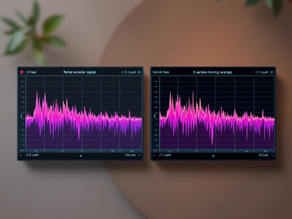
Moving averages with a window of 3–10 samples are simpler than IIR filters and often sufficient for hobby-grade encoders. For higher-precision work, an exponential moving average with a tuned alpha (typically 0.1–0.3) is standard practice and easier to implement on resource-constrained microcontrollers.

One non-negotiable rule: never filter sensor data without logging both raw and filtered streams during development. You need to see what the filter is hiding. A filter that perfectly smooths a 50 Hz buzz might also be hiding a real 2 Hz mechanical resonance you needed to know about. Log both. Always.

Control System Diagnostic Framework

The ten-item operational artifact below is what to run through whenever a control loop misbehaves, in this order. Most problems surface in the first four steps.

1. Plot before you adjust. No serial plotter, no diagnosis. If you cannot see what the loop is doing, you cannot fix it.

2. Test static hold first. Error signal at zero command tells you whether noise or tuning is the issue. Five minutes of static-hold logging often eliminates half the diagnostic tree.

3. Verify mechanical repeatability. Move the joint by hand. Does it return to the same position? If the answer is "approximately," tuning cannot save you. Backlash and flex propagate into every loop downstream.

4. Check loop rate against motor bandwidth. A 50 Hz loop on a 200 Hz motor will oscillate regardless of gains. The Nyquist limit is not a suggestion — your sample rate must exceed 2× the highest frequency component you intend to control, and 5–10× is the practical minimum for clean response.

5. Confirm sensor resolution exceeds tracking requirement by at least 4×. You cannot track tighter than your encoder resolves. A 1024-count encoder on a direct-drive joint gives roughly 0.35° per count — fine for many applications, useless for sub-tenth-degree precision.

6. Validate gains across the full operating envelope. Tune at worst-case voltage, load, and temperature. Validate at best-case. The opposite ordering produces controllers that work in the lab and fail on the floor.

7. Implement integral clamping before deployment. Windup will eventually happen — a stall, a hard stop, an unexpected obstruction. Design for it now. Adding clamping after a field failure is much more expensive than adding it at commissioning.

8. Filter the derivative term, not raw position. Protect against noise without sacrificing P-term response. This is one of the highest-leverage code changes you can make on a noisy system.

9. Log raw and processed signals during commissioning. You cannot debug what you did not record. Build logging in from day one; do not bolt it on after a problem appears, because the problem you most need to debug is the one that already happened.

10. Commit gains to version control with hardware revision. Tuning is engineering data, not folklore. Tag the commit with motor part numbers, sensor revisions, supply voltage, and ambient conditions. Future-you will be grateful, and anyone else maintaining the system will be able to reproduce your work instead of starting over.