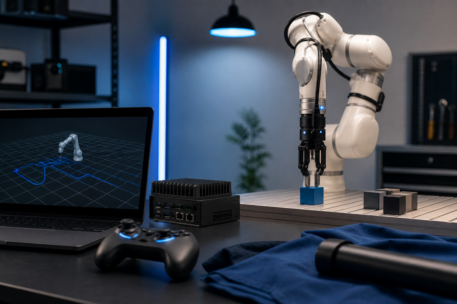
Residual Reinforcement Learning for Robot Control: Combining Classical Controllers with RL Policies

Your team spent six months tuning a PID stack and inverse kinematics solver for a Franka Emika manipulator running PCB assembly. The numbers were excellent: 99.2% first-attempt insertion success across a 14,000-cycle validation run. Then your supplier shipped a batch of boards with a 0.3mm thickness variance, and success collapsed to 71% overnight. The contact phase that worked perfectly against the nominal geometry now produces missed insertions, wedged pins, and the occasional torque-fault recovery.
You face the same fork every contact-rich robotics program eventually hits. Option one: another two months retuning gains, contact thresholds, and approach trajectories for the new tolerance band. Option two: tear out the classical stack and attempt full reinforcement learning from scratch — four to six weeks of simulation training, an uncertain sim-to-real transfer, and no fallback when something goes sideways in production.
There is a third path. It is called residual reinforcement learning for robot control, and it is how teams keep the controllers they already trust while teaching robots to adapt in hours instead of months.
Table of Contents
- Why Classical Controllers Plateau When Tasks or Environments Shift
- How Residual RL Works: Classical Baseline Plus a Learned Correction
- When Residual RL Beats Full RL or Classical Control Alone
- The Real-to-Sim Pipeline That Feeds Residual RL Training
- Why Residual RL Converges 10–100x Faster Than Full RL
- Deploying Residual RL: Pretrained Policies, Edge Hardware, Safe Rollback
- Residual RL Implementation Questions Teams Ask Before Production
Why Classical Controllers Plateau When Tasks or Environments Shift
Classical control is not the villain in this story. PID loops, computed-torque control, and operational-space inverse kinematics dominate industrial robotics because they are built on closed-form models of robot dynamics. They offer provable stability through Lyapunov analysis, deterministic behavior under load, and millisecond-level loop closure that real-time control engineers can audit line by line. PID handles single-DOF position and velocity tracking with predictable phase margins. Trajectory optimizers like CHOMP and STOMP handle obstacle-aware path planning with cost functionals you can inspect. Inverse kinematics — analytical for low-DOF arms, numerical Jacobian-based for redundant manipulators — handles end-effector pose targeting with bounded numerical error. These methods are certifiable, debuggable, and they fail in ways your senior controls engineer can diagnose at a whiteboard.
The break appears when the world stops behaving like the model. Contact-rich tasks — insertion, assembly, in-hand manipulation, deformable-object grasping — assume known contact geometry, but real contact is stochastic. A connector that mates cleanly at 23°C binds at 31°C because the housing expanded 40 microns. Payload variability undoes another set of assumptions: a gripper tuned for 200g objects oscillates at 350g because the inertial gains were never scheduled for that mass. Environmental drift compounds the problem: lighting changes affecting visual servoing, surface friction shifting on a quadruped's foot as humidity climbs, conveyor speed variance in pick-and-place that walks outside the controller's design envelope. And the worst case is multi-task generalization — a classical stack tuned for Task A typically requires near-complete redesign for Task B, because the gain schedules, contact models, and trajectory libraries were specialized to the original task.
The cost of re-tuning is where the economics get ugly. Industrial integrators commonly budget two to six weeks per task variant for classical controller retuning, and that estimate assumes the controls engineer is already familiar with the platform. Loaded engineering cost in U.S. markets runs $150–250/hour for senior robotics talent, which puts a single variant retune in the $30,000–$80,000 range before you count downtime on the cell. Worse, re-tuning is non-transferable: the work doesn't compound across robots or sites, and it doesn't carry over when the next SKU lands.
Re-tuning a classical controller for every new task variant is engineering debt that compounds — every new SKU, payload, or site reset starts the clock over.
The obvious counter — "just use full RL" — runs into its own wall. Full RL training from scratch on contact-rich manipulation routinely requires 10^6 to 10^7 environment interactions to converge, which translates to weeks of simulation time even on parallelized clusters. The sim-to-real gap is brutal: policies trained purely in simulation often degrade 20–40% on real hardware without aggressive domain randomization, and even with it, transfer remains the dominant source of project risk. There is no safety fallback — if a fully trained RL policy fails in production, there is no clean handoff to a stable controller, only a fault-stop and a human in the loop. And in regulated environments like medical device assembly or automotive safety-critical lines, opaque end-to-end neural policies will not be accepted as the sole control law. The certification story does not close.
So you are stuck choosing between rigid-but-certifiable and flexible-but-unaccountable. That framing is a false dichotomy. The architecture that resolves the trade-off does not replace your classical stack. It augments it.
How Residual RL Works: Classical Baseline Plus a Learned Correction
Residual RL is structurally simple: the final action sent to the robot is the sum of a classical controller's output and a small corrective signal produced by a neural network policy. Formally, a_total = a_classical(s) + a_residual(s; θ), where θ is trained via standard reinforcement learning algorithms — PPO, SAC, or TD3 — to minimize task cost. The classical controller is frozen. Only the residual is learned.
| Dimension | Classical Control Only | Full RL (End-to-End) | Residual RL |
|---|---|---|---|
| Training samples | 0 (analytical) | 10^6–10^7 steps | 10^4–10^5 steps |
| Time to deploy | Weeks of manual tuning | 2–8 weeks training | Hours to days |
| Stability guarantees | Provable (Lyapunov) | None inherent | Inherits baseline within bounded residual |
| Sim-to-real risk | N/A | High (20–40% drop) | Low (small corrections) |
| Rollback | N/A | Replace policy | Disable residual → revert instantly |
| Action space | None | Full motor command space | Bounded ±10–20% of action range |
| Best fit | Static, well-modeled | No prior controller | Baseline exists, environment varies |
The residual is bounded by design. Most implementations clip the residual output to a fraction — commonly 10–20% — of the total action range. That clip is what gives residual RL its safety profile: the RL policy cannot override the classical controller during exploration, because the magnitude of any single correction is constrained. Even a maximally adversarial residual produces only a bounded perturbation around a known-stable baseline trajectory.
Walk through a concrete peg-in-hole insertion on a Franka manipulator. The classical impedance controller sets the desired end-effector pose and stiffness across the entire motion. The residual RL policy observes force/torque sensor readings from the wrist sensor and outputs micro-adjustments — sub-millimeter pose deltas and stiffness modulations — that fire only during the contact-rich phase. The classical controller still owns approach and retraction; the residual contributes only during the uncertain contact window, where the analytical model is weakest. The residual is not learning the task. It is learning the error model between what the classical controller predicts and what the environment actually requires — a far lower-dimensional learning problem than learning insertion from scratch.
Network size follows from the simpler objective. Residual policies typically run 500K to 2M parameters, against 10M–100M for end-to-end policies. That compactness matters at deployment: a sub-1M-parameter residual network runs comfortably on edge hardware like the Kinematics Mini's Jetson Orin Nano (40 TOPS) inside a 50ms control loop without latency penalty. The foundational work here traces to Johannink et al. at Berkeley (2019) and Silver et al. at MIT (2018), who formalized residual policy learning as a way to combine model-based priors with learned corrections — research that has since been validated across manipulation, locomotion, and aerial control benchmarks.
When Residual RL Beats Full RL or Classical Control Alone
Residual RL is not universally the right answer. It excels in a specific quadrant: tasks where a reasonable classical baseline exists and the environment has bounded but unpredictable variability. The decision matrix below maps common robotics use cases to the architecture that fits each.
| Use Case | Classical Only | Full RL | Residual RL |
|---|---|---|---|
| Static pick-and-place, fixed parts | ✅ Optimal | ⚠️ Overkill | ⚠️ Unnecessary |
| Assembly with part variance | ❌ Brittle | ⚠️ Slow to deploy | ✅ Optimal |
| In-hand manipulation, deformables | ❌ Inadequate | ✅ Justified | ✅ Optimal if baseline exists |
| Quadruped on known terrain | ✅ Adequate | ⚠️ Overkill | ✅ Optimal for adaptation |
| Quadruped on unknown rough terrain | ❌ Fails | ✅ Justified | ✅ Optimal with gait baseline |
| Humanoid whole-body balance | ❌ Fragile | ⚠️ Sample-hungry | ✅ Optimal (LIPM + residual) |
| Mobile robot, dynamic obstacles | ⚠️ Reactive only | ⚠️ Slow | ✅ Optimal (planner + residual) |
The matrix logic comes down to two conditions. Residual RL wins wherever a baseline controller produces 70–90% of the desired behavior, and the remaining 10–30% is structured variability that benefits from learning. Outside that quadrant, the architecture either adds unnecessary complexity (when classical alone suffices) or asks too little of the network (when the baseline is so weak that the residual must do most of the work).
Consider the assembly case in detail. A Franka manipulator inserting board-to-board connectors with 0.5mm position variance and 0.2N force variance cannot be handled cleanly by impedance control alone, because the contact phase has more uncertainty than the controller's gain schedule was tuned for. Classical impedance handles the gross approach. The residual policy learns to modulate stiffness during the final 5mm of contact-rich approach, observing the force-torque signal and emitting sub-millimeter corrections. Training converges in roughly two hours of cloud simulation time on a single GPU, against four to six weeks for an end-to-end policy that would have to learn approach, contact, and retraction from scratch.
The quadruped case has the same shape. A Unitree Go2 running model-predictive control produces a clean trot on flat ground but trips on an 8cm rock because the MPC's footstep planner does not know what the rock is. Residual RL adds stride-length and foot-placement corrections triggered by IMU and proprioceptive signals, trained in domain-randomized terrain simulation. The MPC gait stays intact and certifiable. The residual handles the structured-but-noisy reality the gait planner cannot see.
Warehouse mobile robots show the same pattern at navigation scale. A global path planner — A*, RRT*, or any of the standard ROS2 navigation stacks — handles the route. The residual handles micro-adjustments for human pedestrians who do not behave like the obstacle-avoidance assumptions baked into the planner. The global plan stays auditable. The local behavior adapts.
When is full RL still correct? When you have no usable baseline. Learning a genuinely novel tool-use skill with no prior dynamics model — a new surgical instrument, a new compliant gripper geometry — gives you nothing to be residual to, and the architecture loses its sample-efficiency advantage. And when is classical alone correct? When the environment is fully characterized and unchanging. A CNC tending robot with fixed part presentation, repeatable fixturing, and stable thermal conditions does not justify the overhead of training and managing an RL policy, however small.
The OpenKinematics fit lands cleanly here: the platform's pretrained policy library — manipulation primitives, quadruped gaits, humanoid balance — serves as the baseline in residual RL workflows. Teams skip the baseline-design step entirely and train only the residual against their specific site, payload, and task variant.
The Real-to-Sim Pipeline That Feeds Residual RL Training
Residual RL training requires a simulation environment that matches your deployment site closely enough that the small corrections learned in sim survive transfer to hardware. The pipeline below is how teams get from physical workspace to trained residual policy, sim-to-real risk minimized at every step.
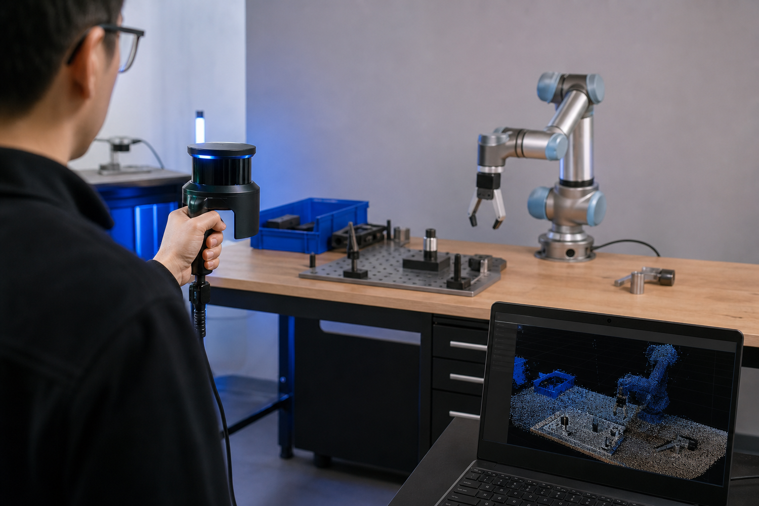
Step 1 — Capture the workspace with LiDAR (5–15 minutes). Use a handheld or robot-mounted LiDAR — a Livox Mid-360 class sensor is typical — to scan the physical workspace. Output is a dense point cloud of fixed geometry: tables, fixtures, conveyors, shelving, racking. This step replaces what used to be one to three weeks of manual CAD modeling and fixture measurement.
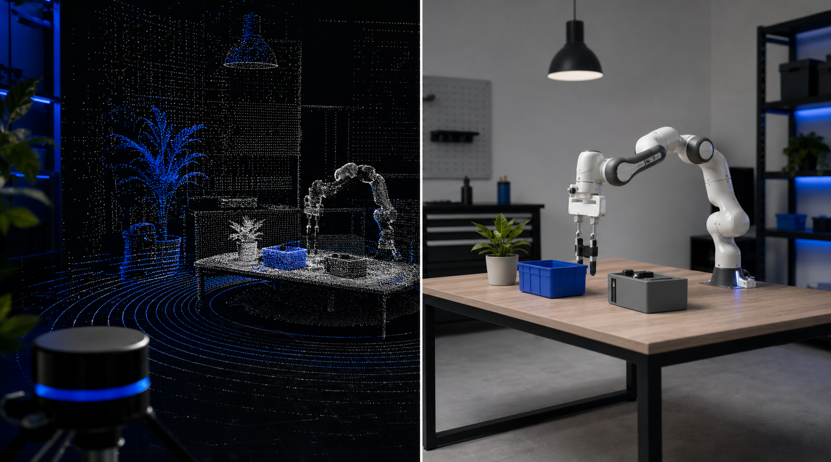
Step 2 — Generate the digital twin (automated, minutes). The point cloud is processed into a simulation-ready mesh with collision geometry. Articulated objects (doors, bins, hinged covers) and dynamic objects (parts, tools, fixtures that move) are tagged for physics simulation. The output is an Isaac Sim or MuJoCo-compatible scene that matches site geometry to a few millimeters.
Step 3 — Drop in the classical baseline controller. Load the existing PID, MPC, or impedance controller — or select a pretrained policy from the cap-x library. This becomes the frozen baseline that residual RL will modify. It is never retrained. Its action outputs are sampled at every control step alongside the residual.
Step 4 — Define the residual policy network and reward. Specify a small neural network — typically two to three hidden layers, 256 to 512 units per layer — that takes state observations and outputs bounded action deltas. The reward function encodes task success: placement accuracy, force limits, time efficiency, energy budget. Reward shaping is lighter than in end-to-end RL because the baseline already achieves most of the task.
Step 5 — Train in cloud simulation with domain randomization (minutes to hours). Run PPO or SAC across parallelized simulation instances — often 256 to 1,024 parallel environments. Domain randomization varies friction coefficients, mass, contact stiffness, sensor noise, and actuator latency so the residual generalizes across the variation envelope you expect at deployment. Convergence typically lands at 10^4 to 10^5 episodes.
Step 6 — One-click deployment to edge hardware. The trained residual policy and frozen baseline are packaged and pushed to the OpenBrain edge stack. The classical baseline executes in the real-time control loop. The residual runs as an additive corrective signal, with disable-on-fault built in at the runtime level.

Why Residual RL Converges 10–100x Faster Than Full RL
The single most important practical advantage of residual reinforcement learning for robot control is sample efficiency. Where full RL on contact-rich manipulation routinely requires 10^6 to 10^7 environment steps, residual RL converges in 10^4 to 10^5 steps on the same tasks. Five mechanisms drive that two-to-three-orders-of-magnitude gap in data efficiency for RL training.
- Compressed action space. The residual policy outputs small deltas, often clipped to ±15% of the full action range, rather than absolute motor commands. A smaller output space means fewer parameters need optimization, exploration noise stays inside safe bounds even early in training, and the gradient signal from the reward concentrates on a much smaller manifold of useful corrections.
- Pre-shaped reward landscape. The classical baseline already achieves 70–90% of task reward on its own. The RL policy starts optimization near the reward surface's good neighborhood rather than at random initialization. There are far fewer poor local minima to escape because the baseline has already done the hard work of getting close to a solution. The residual fills the gap, not the chasm.
- Reduced sim-to-real gap. Small corrective actions are inherently less sensitive to dynamics mismatch than full action trajectories. If simulated friction differs from real friction by 15%, a full RL policy's entire learned trajectory drifts; a residual policy's small correction shifts only marginally, because the baseline controller absorbs most of the model error. This is the structural reason RL convergence in sim translates more reliably to hardware behavior.
- Faster early stopping. Teams routinely stop residual RL training when the policy reaches 90–95% of asymptotic performance, because the classical baseline guarantees a safe floor. Full RL has no such floor — you cannot stop early without risking deployment of an incompletely-trained policy that may behave pathologically on out-of-distribution states.
- Network size and inference cost. Residual policies typically run 500K to 2M parameters versus 10M to 100M for end-to-end policies. They train faster per step, transfer more easily to edge hardware, and meet real-time loop budgets (sub-50ms) on Jetson Orin Nano-class compute without quantization tricks.
Residual RL doesn't ask the network to invent control from scratch. It asks only where the classical controller is wrong, and by how much — a vastly easier question to answer.
Translated to deployment timelines: a manipulation skill that would require four to six weeks of full RL training plus two weeks of sim-to-real validation collapses to a single afternoon of cloud training plus deployment. For teams using cloud simulation and one-click hardware push, the end-to-end timeline from environment scan to deployed residual policy fits inside the roughly 60-minute window the OpenKinematics platform is designed around.

Deploying Residual RL: Pretrained Policies, Edge Hardware, Safe Rollback
Residual reinforcement learning for robot control is only valuable if you can ship it. Three architectural properties — pretrained baselines, deterministic edge execution, and non-destructive rollback — determine whether a residual policy survives the trip from cloud training to a working cell.
Pretrained Policies as the Frozen Baseline
The cap-x framework ships pretrained RL policies for high-frequency task families: 6-DOF pick-and-place, planar push, in-hand reorientation, quadruped trot and walk gaits, and bipedal balance primitives. In a residual RL workflow, these pretrained policies serve as the frozen baseline. Teams do not retrain them. Instead, they train a small residual network that adapts the pretrained policy to the specific site, payload, or task variant in front of them.
Contrast that with the alternative approaches in the field. Covariant, Skild, and Intrinsic generally fine-tune large foundation policies for each customer, which requires either substantial data collection on customer hardware or long retraining cycles measured in days or weeks. Residual RL on cap-x skips both: the foundation policy stays fixed, and only the small residual is site-specific. A customer deploying the pick-and-place skill on a new conveyor with new SKUs trains a residual in hours, not the days-to-weeks required by fine-tuning approaches. The pretrained policy carries 80% of the behavior across deployments; the residual carries the last 20% that is genuinely unique to the site.
Edge Execution on Kinematics Mini and Max
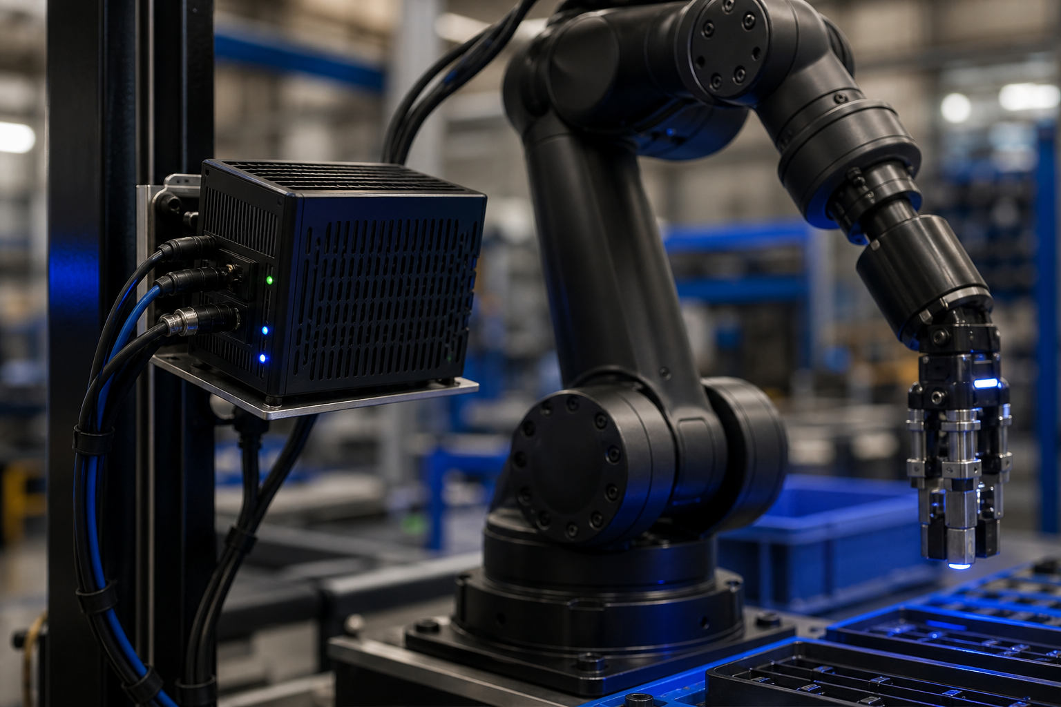
The Kinematics Mini is an NVIDIA Jetson Orin Nano-based edge unit at $1,499, built on an open-source hardware design. It offers 40 TOPS of AI compute — sufficient to run both a pretrained baseline policy and a residual network in the same 50ms control loop with headroom for vision preprocessing. The Kinematics Max is the industrial enclosure variant built around Jetson AGX Orin or T4000/T5000 modules, sized for fleet operations and higher-DOF systems including humanoids and multi-arm cells where the action space and observation rate demand more silicon.
The OpenBrain edge stack — MIT-licensed and open — handles deterministic scheduling. The classical baseline runs as a hard real-time process with guaranteed timing. The residual policy inference runs as a soft real-time process with bounded latency. If residual inference exceeds its time budget on any given control step, the system falls back to baseline-only output rather than missing the control deadline. The robot keeps moving under the certifiable controller; the learned correction simply skips a cycle. This is the property that lets residual RL coexist with safety-rated control loops.
Hardware-agnostic integration is the other half of the deployment story. Native ROS2 bridges connect to Unitree quadrupeds, Franka manipulators, and Universal Robots arms. The same residual policy artifact runs across compatible robot platforms because cap-x abstracts the action space at the controller-output level — you train once against the action interface and deploy across hardware that conforms to it.
Safety Rails and Iterative Rollout
The residual policy can be disabled via a runtime flag without restarting the classical controller. That single property enables phased deployment in a way end-to-end RL cannot match: run baseline-only for the first production week, activate residual corrections in week two as confidence builds, monitor the performance deltas in detail. A/B comparison is direct — alternate residual on/off across shifts and compare success rates, cycle times, and force-fault counts side by side.
Rollback in residual RL is non-destructive. Because the baseline is unchanged, rolling back to a prior residual version, or disabling the residual entirely, returns the robot to a known-good control law instantly. There is no policy-swap warm-up period, no risk of an intermediate state with mixed behavior. The classical controller carries the safety case across rollbacks; the residual is an additive enhancement that can be audited as a bounded perturbation around an approved baseline.
This is the architectural property that makes residual RL compatible with regulated environments where end-to-end neural policies cannot be certified. The certification artifact is the classical controller plus a bounded perturbation envelope. The residual lives inside that envelope.
Residual RL earns trust in deployment because you're not betting the robot on an untested neural network — you're adding a small, bounded, interpretable correction to a controller you already know works.
Residual RL Implementation Questions Teams Ask Before Production
Can I use residual RL with non-RL baselines like model predictive control or learning-from-demonstration policies?
Yes. The residual architecture is agnostic to baseline type — what matters is that the baseline produces actions in the same space the residual outputs corrections to. MPC controllers, behavioral cloning policies, diffusion policies, and analytical inverse-dynamics controllers all work as baselines. The only structural requirement is that you can sample the baseline's action at every control step, so the residual has something to add to. In practice, MPC plus residual RL is one of the most common pairings for legged locomotion, where the MPC handles gait scheduling and the residual handles terrain adaptation. Behavioral-cloning plus residual RL is common for manipulation tasks where human teleoperation demonstrations provide a strong starting baseline.
How do I know if my residual RL policy has converged enough for hardware deployment?
Three signals matter. First, reward curve plateau on validation episodes — improvement under 1% over 1,000 episodes indicates convergence has stabilized. Second, residual magnitude statistics: the average residual action should stabilize and stay well below the action clip threshold, typically below 50% of clip range, indicating the policy is not pushing against its bounds. If the residual is saturated against the clip, your action range is undersized or your baseline is too weak. Third, a small live trial on hardware — 10 to 50 episodes — confirming sim-to-real transfer with under 5% performance drop versus simulation results. If all three hold simultaneously, the policy is deployment-ready.
What happens if my classical baseline is poor? Does residual RL still work?
It works, but it loses its efficiency advantage. If the baseline achieves only 30–40% of task performance, the residual must learn larger corrections, which expands the effective action space and pushes sample requirements toward full-RL territory of 10^6 or more steps. Worse, large residuals erode the safety story — if the residual is doing most of the work, the classical fallback no longer guarantees acceptable behavior on rollback. The interpretability argument collapses with it. Best practice: invest a few days tuning the classical baseline to at least 60–70% task performance before training the residual. That investment pays back many times over in training time, deployment confidence, and certification clarity.
Can I combine residual RL with domain randomization and other sim-to-real techniques?
Yes, and you should. Domain randomization during residual training broadens the baseline's effective robustness without changing the baseline itself. The residual learns to compensate for the worst-case randomized dynamics, which makes the deployed policy resilient to real-world variation in friction, mass, sensor noise, and actuator delay. Other compatible techniques: privileged information distillation (train with full sim state, deploy with partial observation), system identification (calibrate sim parameters from real data logs), and adversarial perturbations during training to harden the residual against worst-case inputs. These techniques compound with residual RL rather than competing with it — each one reduces a different component of the sim-to-real transfer error, and the residual's bounded action range amplifies their effect because small corrections degrade gracefully when any single technique falls short.