Computer Vision in Robotics: How Perception Powers Modern Autonomous Systems

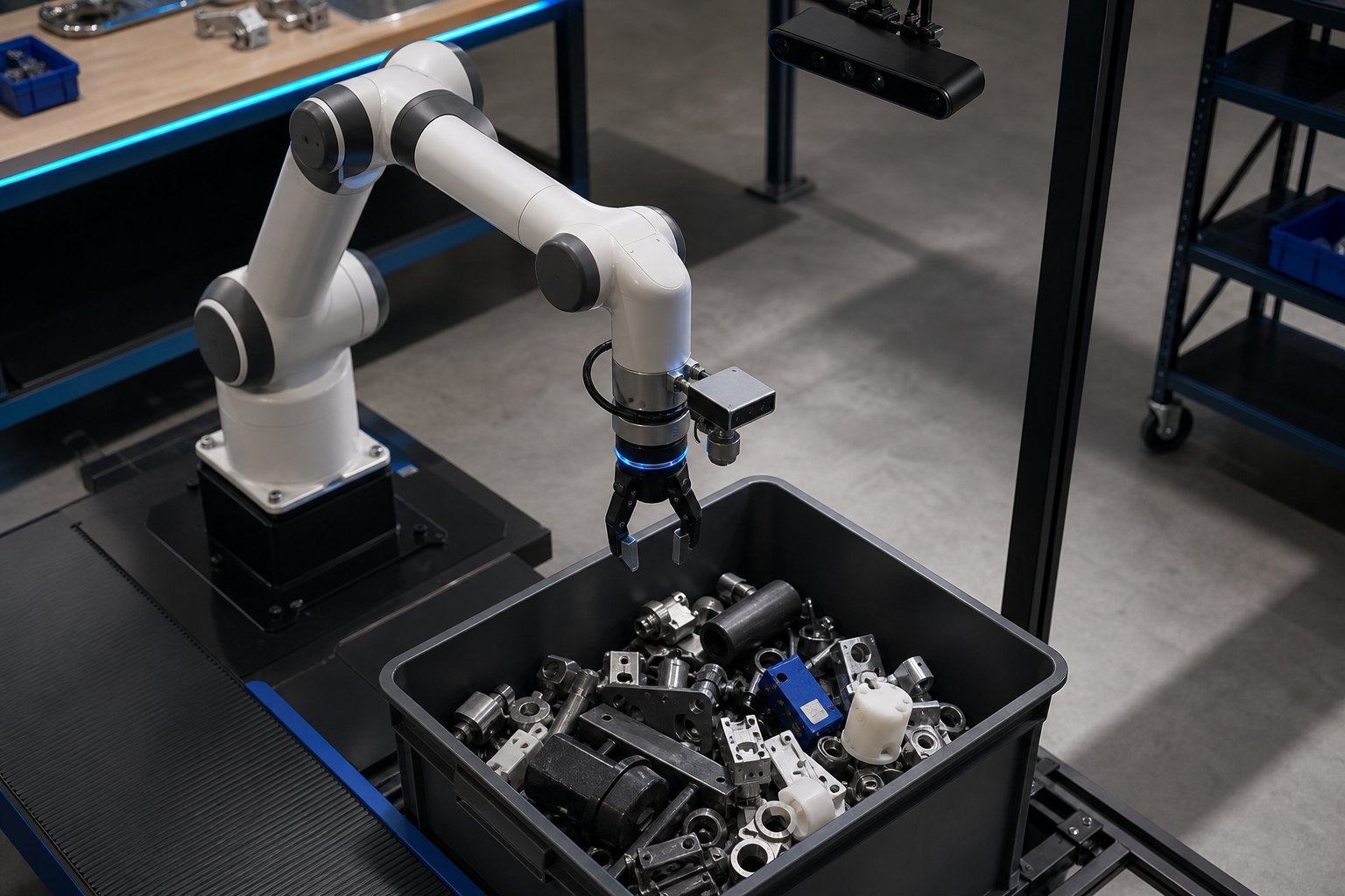
You have probably watched it happen on your own factory floor. A six-axis arm that can repeat a trajectory to within 0.05 mm sits idle because an incoming tote arrived with parts oriented 20° off-template, and the hard-coded grasp routine refuses to fire. Every minute that arm stays down costs money, and the failure is not mechanical — it is perceptual. The robot can move; it cannot interpret. Computer vision in robotics is the layer that closes that gap, translating pixels into semantic decisions a control loop can actually use.

Every robotics team eventually hits the same wall. Proprioception, force feedback, and LiDAR geometry are sufficient inside tightly fixtured cells. They collapse the moment the environment varies. Vision systems provide object detection, depth perception, and pattern recognition that let robots identify objects, assess surroundings, and make real-time decisions in dynamic environments, according to Ultralytics and the peer-reviewed Robotics Perception and Control survey. This article is a practitioner walk-through of how that layer actually works, where it breaks, which architectures fit which constraints, and what to validate before you ship.

Table of Contents

• Why Robot Perception Collapses Without Computer Vision
• The Three Layers of Vision: Traditional CV, Deep Learning, and Multimodal Fusion
• Canonical Vision Tasks in Robotics
• Matching Vision Architecture to Hardware and Latency Budget
• From Environment Capture to Deployed Skill: The Real-to-Sim-to-Real Pipeline
• Why Vision Models Fail on Real Hardware: The Sim-to-Real Gap
• Pre-Deployment Validation Checklist for Vision-Enabled Robots
• Five Failure Patterns That Sink Vision-Enabled Robotics Programs

Why Robot Perception Collapses Without Computer Vision

Robot perception is formally the task of making sense of an unstructured world from incomplete, noisy sensory data, then feeding state estimation and control. That definition comes straight out of the UT Austin CS391R Robot Perception lectures and is echoed in the Michigan Robotics perception research area overview. Vision is one primary modality alongside LiDAR, IMU, and proprioception — but it is the modality that carries semantic information no range sensor can produce. A point cloud tells you a surface exists at 1.2 m. Only a camera tells you that surface is the back of a forklift, a person, or a stack of mislabeled crates.

The performance delta is not subtle. Surveyed robot perception work reports that adding visual perception to robots using only proprioception or range sensing improves success rates on navigation and manipulation benchmarks from roughly 60–70% to over 90% in structured settings, and is critical to reaching usable performance in unstructured environments, per the Robotics Perception and Control survey and the practitioner-facing arXiv 2112.05534. Inside a fixtured cell, that gap is annoying. Outside one, it is the difference between a robot that runs and a robot that does not.

Three concrete failure modes show up over and over when vision is absent or thin:

• Bin picking without object segmentation. Point-cloud depth alone cannot reliably distinguish two adjacent identical parts. The gripper picks the gap between them — or pinches both — and the task fails silently. The Vision for Robotics CS545 notes treat instance segmentation as the standard remedy.
• Navigation on reflective or transparent surfaces. LiDAR returns degrade on glass partitions, polished concrete, and dark mats. Only vision can interpret those surfaces semantically — "that is a glass door, not free space" — as the Robotics Perception and Control survey makes explicit.
• Assembly under variable pose. Pre-programmed offsets fail when an incoming part is rotated 15° beyond expected tolerance. Without edge or feature detection, force feedback alone produces a collision before the correction signal arrives.

There is a tempting counter-argument: dead reckoning plus force feedback was enough for industrial robotics through the 1990s and 2000s, so why bolt on the complexity of a vision stack now? Miguel Valencia answers this directly in the UQCS "How Robots See" talk: "what good is a robot if it can't actually interact with the real world?" The 1990s model worked because every variant was fixtured, every part was presented in the same pose, and every cell was custom-engineered. The moment you need to handle SKU variation, mobile platforms, or human-shared workspaces, the cost of fixturing every case equals or exceeds the cost of adding vision — and fixturing does not scale with product mix the way a retrainable model does.

A robot without vision is a robot that works in one environment, at one time of day, performing one task. Scale any of those variables and it fails silently — usually right after acceptance testing.

The practitioner question is not whether vision belongs in modern robotics. It is which vision approach fits which task, hardware, and latency budget — and how you get from environment capture to a deployed model without spending a year on labeling. The rest of this article works through that decision, layer by layer.

The Three Layers of Vision: Traditional CV, Deep Learning, and Multimodal Fusion

Three dominant vision architecture classes compete for the same robot perception slot, and they sit on very different points of the latency-robustness-cost curve. Educational and survey sources — the UQCS talk, the Vision for Robotics notes, and Michigan Robotics — converge on the same taxonomy: traditional CV (edge detection, color thresholding, template matching) is low-latency but brittle; deep CNNs and transformers are higher-latency but robust to variance; and multimodal fusion combines vision with LiDAR, IMU, or tactile signals for the highest robustness at the highest compute cost.

Approach	Typical Latency	Training Data	Robustness	Compute Profile
Traditional CV	Single-digit to tens of ms	None (rule-based tuning)	Low — fails on lighting/viewpoint shifts	CPU or low-end edge
Deep Learning (CNN, ViT)	Tens of ms (CNN) to hundreds (ViT)	Hundreds to thousands of labeled images	High within trained distribution	Edge GPU (Jetson Orin class) or cloud
Multimodal Fusion	Tens to hundreds of ms	Deep learning data + sensor calibration	Highest — redundancy covers single-modality failure	Edge GPU + sensor sync stack

Latency ranges drawn from the CS545 Vision for Robotics notes, the Robotics Perception and Control survey, and arXiv 2112.05534. Data requirements from UT Austin CS391R.

Traditional CV still wins in narrow, controlled environments. Fixtured assembly with fiducial markers, color-coded sorting on conveyors, barcode and QR-driven pick stations — these are the domains where hand-crafted features outperform anything deep learning can offer. Inference fits inside single-digit milliseconds, no training data is needed, and the brittleness is acceptable because the environment never varies. The UQCS talk is blunt about this: if you can lock down the lighting and pose, you do not need a neural network.

Deep learning dominates every new deployment that exits the fixtured cell. Once parts arrive in random orientations, or operators share the workspace, or lighting changes across a shift, hand-crafted features collapse. CNN detectors deliver high accuracy on trained classes with tens of ms inference on Jetson-class hardware. The cost is data — hundreds to thousands of labeled images per task in the conventional regime, according to the UT Austin CS391R lectures — and that data is where most projects stall.

Multimodal fusion is now the default for serious deployments. University robotics programs and the Robotics Perception and Control survey both highlight fusion as a central research focus rather than an edge case. RGB fails in low light. Depth fails on reflective surfaces. LiDAR struggles with transparent object detection. Combining modalities is how you remove single points of failure, and it is the only path to the kind of reliability industrial buyers will sign off on. The trade-off is sensor synchronization, calibration overhead, and a fusion architecture that has to be designed — not something you bolt on after the fact.

The practitioner heuristic worth memorizing: match the approach to the variance in your deployment environment, not the sophistication of the team building it. A simpler stack that handles your actual variance beats a transformer that handles variance you do not have.

Canonical Vision Tasks in Robotics

Robotics teaching material standardizes four core visual tasks underpinning every manipulation and navigation vision pipeline: detection, segmentation, classification, and pose estimation, with deep CNNs as the dominant technical baseline. That structure is consistent across the UQCS talk, the Vision for Robotics notes, and the Robotics Perception and Control survey. Understanding what each task does — and where it stops working — is how you avoid asking a detector to do a segmenter's job.

• Object Detection — "what is here, and where." Output: 2D bounding boxes with class labels and confidence scores. Used for identifying graspable items in a bin, locating fiducials, spotting humans in collaborative workspaces. Standard models are YOLOv8, Faster R-CNN, and Detectron2. Latency on Jetson-class edge GPUs falls in the tens of ms range. The failure mode is geometric coarseness: bounding boxes tell you what is there but not the precise contour or orientation needed for a precision grasp. For a tote of touching identical parts, object detection alone is not enough.
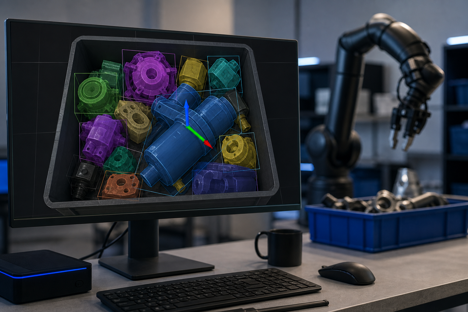
• Semantic and Instance Segmentation — "draw the outline of every object." Output: per-pixel class labels (semantic) or per-pixel instance IDs (instance). Used for separating touching parts in a tote, distinguishing floor from clutter for mobile robots, and generating clean grasp regions. Standard models include Mask R-CNN and SAM (Segment Anything). SAM in particular enables zero-shot segmentation without task-specific training, which the UT Austin CS391R lectures flag as a meaningful shift in how teams approach annotation cost.
• 6-DoF Pose Estimation — "what orientation is it in." Output: full 6-degree-of-freedom pose (x, y, z, roll, pitch, yaw) of the target object relative to the camera or robot base. Pose estimation is the task that converts a detected object into an executable grasp plan. Standard approaches include PoseCNN, FoundationPose, and point-cloud registration. The dominant failure mode is symmetry: symmetric objects produce pose ambiguity that downstream control must handle explicitly, or the gripper will rotate to a valid pose that is nevertheless the wrong one.
• Tracking and Visual Servoing — "follow the target across frames." Output: object identity persistence across a video stream, used to close the perception-action loop. Robot perception curricula treat perception as active and embodied — the robot moves to gather better views — which underpins visual servoing and closed-loop vision-based control, per UT Austin CS391R and Michigan Robotics. Tracking is what turns a single-frame detector into a manipulation system that can respond to a moving target.

Most production pipelines chain these tasks. Detection narrows the field of view, segmentation isolates the target, pose estimation defines the grasp, and tracking maintains it as the robot moves. Treating any single task as the whole pipeline is how you end up shipping a demo that does not survive contact with a real bin.

Matching Vision Architecture to Hardware and Latency Budget

Architecture selection for computer vision in robotics is constraint matching. Teams work backwards from two numbers: the control loop period and the available edge compute. Closed-loop control commonly runs at 10–100 Hz, implying vision must either fit inside a 10–100 ms cycle or run asynchronously with motion prediction to avoid instability, per the UT Austin CS391R lectures and arXiv 2112.05534. Pick the architecture that fits those numbers — not the one that benchmarks best on a workstation.

• Convolutional Neural Networks (CNNs) — the workhorse. Best for object detection, segmentation, and pose estimation with well-defined classes. Hardware: Jetson Orin Nano at the entry edge, Orin / T4000 / T5000 at the production edge. Latency: tens of ms per frame on edge GPUs. Data: hundreds to thousands of labeled examples per task. Choose CNNs when the task is bounded, you can collect or generate the data, and your control loop tolerates 30–100 ms vision latency. This is the default for bin picking, pick-and-place, and inspection, supported by the Robotics Perception and Control survey and arXiv 2112.05534.
• Vision Transformers and Foundation Models — the flexibility option. Best for open-vocabulary detection ("pick any red object"), few-shot adaptation, and semantic understanding of novel scenes. Models include CLIP, SAM, DINO, and vision-language models. Hardware: Orin Nano struggles; Orin AGX or cloud edge inference is recommended. Latency: hundreds of ms on edge, faster in cloud. Data: tens of labeled examples for fine-tuning, using massive generic pretraining. Choose foundation models when task definitions shift, deployment environments vary, or you cannot afford to retrain a CNN per SKU change.
• Lightweight Models (MobileNet, TinyYOLO, quantized CNNs) — the real-time option. Best for high-frame-rate perception on constrained hardware. Hardware: Jetson Orin Nano, mobile SoCs, edge TPUs. Latency: single-digit to low tens of ms. Trade-off: lower accuracy than full-size CNNs and narrower class coverage. Choose lightweight models when you need >30 fps perception, the model must fit in tight memory, or the robot operates without cloud connectivity. The Vision for Robotics notes cover this as the standard real-time tier.
• Multimodal Fusion Stacks — the robustness option. Best for contact-rich manipulation, navigation in adversarial lighting, and safety-critical tasks. Architecture: parallel encoders for RGB, depth/LiDAR, IMU, and tactile, fused via attention or learned projection. Hardware: Jetson Orin AGX or cloud, with synchronized sensor capture. Latency: tens to hundreds of ms depending on fusion strategy. Choose fusion when no single modality covers your environment's failure cases — a position supported by both the Robotics Perception and Control survey and Michigan Robotics.

The fastest vision model is useless if it guesses wrong. The most accurate model is useless if it decides slower than your gripper can move. Architecture selection is constraint matching, not benchmark chasing.

The most common mistake teams make is selecting the model class before profiling edge inference latency on the actual target hardware. A 250 ms transformer feels fine on a workstation. It is unusable on a 100 Hz control loop. Profile first, train second.

From Environment Capture to Deployed Skill: The Real-to-Sim-to-Real Pipeline

Most teams underestimate how much of a vision project is data, not model. Pragmatic guides recommend capturing dozens to a few hundred images of task environments with variation in pose, lighting, and clutter as a practical starting point, supplemented by synthetic data and simulation to expand coverage without exhaustive manual labeling — per the UT Austin CS391R lectures, the Vision for Robotics notes, and arXiv 2112.05534. A real-to-sim-to-real pipeline is how you cut that data problem from a year of labeling to a week of capture.

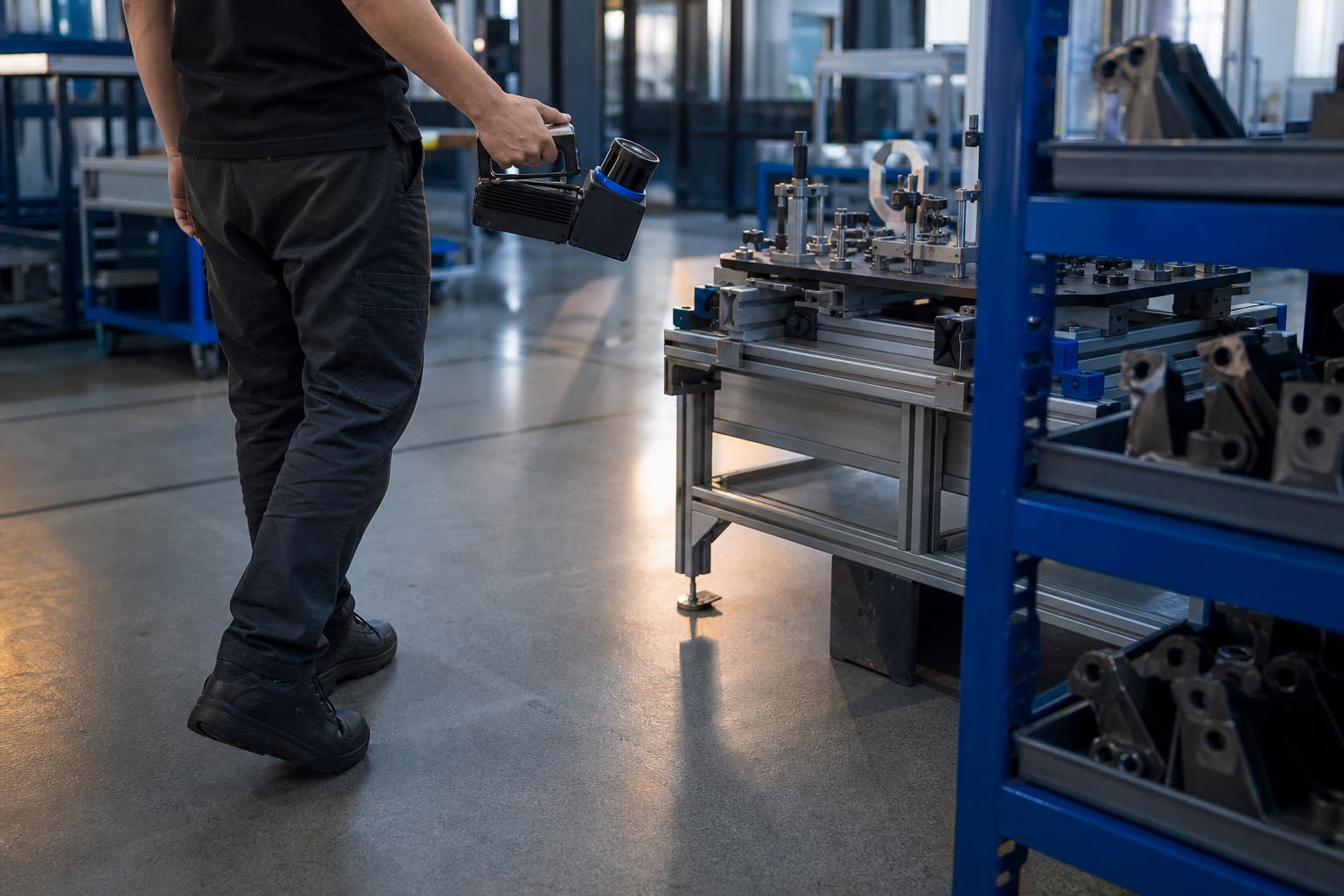
1. Capture the Real Environment. Photos, video, or LiDAR scans of the actual workcell or operating area. Target: 50–200 images covering task variants — different object poses, lighting at different times of day, realistic clutter density. LiDAR adds the geometric scaffold; cameras add appearance. The point of real-to-sim capture is to anchor downstream simulation in the same visual statistics the robot will face at runtime. Skip this step and your simulator is just generating plausible-looking noise. The arXiv pragmatic guide is direct that real anchoring is what makes synthetic generation useful.

   

2. Reconstruct or Augment into Simulation. Convert captures into photogrammetry meshes, NeRF-style reconstructions, or photo-real rendered scenes. Add domain randomization on top: vary lighting, surface textures, object placement, distractors. The Robotics Perception and Control survey and UT Austin CS391R both report sizable accuracy gains when models are trained with domain randomization versus naive sim training. The goal is not photorealism — it is exposing the model to a wider distribution than reality so reality looks like an in-distribution sample.
3. Label Strategically or Use Self-Supervised Proxies. Full manual labeling is only justified when the target class is rare, safety-critical, or unavailable in foundation-model vocabularies. Otherwise: use SAM for zero-shot masks, CLIP for zero-shot classification, or synthetic-data generation where ground truth comes free from the simulator. Conventional CNNs need hundreds to thousands of labeled images. Foundation-model adaptation can work with tens. That ratio decides whether your labeling budget is a week or a quarter.
4. Train the Vision Policy. Three options. Supervised training of a detector or segmenter on labeled data. Self-supervised pretraining followed by light fine-tuning. Or end-to-end reinforcement learning where the vision encoder learns alongside the control policy. RL learns what to look at from reward signals; supervised models require you to define the classes upfront. The Voxel51 talk describes "robot-supervised learning," where the robot uses its own actions and depth estimates to annotate new training data over time, reducing manual labeling burden as the deployment matures.
5. Validate in Sim, Deploy, Iterate on Real Failures. Test with full domain randomization, then progressively narrow toward the deployment distribution. After deployment, log low-confidence predictions and use them as the next training batch. If real-world accuracy is below 80%, retrain on harder sim variants before collecting more real data — the bottleneck is rarely real-data volume, it is sim-coverage breadth.

The pipeline above is the difference between treating vision as a one-shot model delivery and treating it as a continuously improving asset. Teams that build the loop ship faster after deployment. Teams that do not, ship once and slowly watch accuracy decay.

Why Vision Models Fail on Real Hardware: The Sim-to-Real Gap

Robot perception research repeatedly reports that models achieving over 90% detection or segmentation accuracy in simulation can drop to roughly 50–60% when first deployed on real hardware due to the domain gap — lighting, texture, clutter, and sensor noise. That finding is consistent across the UT Austin CS391R lectures, the Robotics Perception and Control survey, and arXiv 2112.05534. This gap is not solved by collecting more real data alone. It is an architectural and training-distribution problem, and computer vision in robotics stands or falls on how seriously a team treats it.

Lighting and appearance variance. Synthetic renderers default to clean directional lighting. Real workcells have mixed fluorescent, daylight bleed-through, and operator shadows that move across the scene every few seconds. A model trained only on default sim lighting can lose 30 or more percentage points of accuracy in deployment. Mitigation at training time is domain randomization — vary brightness, contrast, hue, and shadow geometry across thousands of sim episodes. Mitigation at deployment time is locking camera white balance per location and applying histogram equalization as a preprocessing step. Neither alone is enough; both are cheap.

Clutter, occlusion, and density. Sim scenes are typically sparser than real bins. A detector trained on tidy sim scenes overconfidently predicts on packed totes, returning high-confidence bounding boxes for partially occluded parts that no gripper can actually reach. Architectural mitigation: attention-based architectures reason about partial views better than vanilla CNNs. Training mitigation: aggressively randomize object density and inter-object occlusion in sim. The Robotics Perception and Control survey flags this as one of the most consistent sim-to-real failure modes in industrial deployments.

Motion blur and sensor artifacts. Real cameras face an exposure trade-off: fast shutter freezes motion but darkens the frame; slow shutter brightens but blurs. Add rolling-shutter skew on a fast-moving manipulator and you have artifacts no sim renderer produces by default. Mitigation: synthetic motion-blur augmentation, brightness reduction during training, and at the hardware level, global-shutter industrial cameras for fast manipulators. The arXiv pragmatic guide treats this as a frequently underestimated source of deployment regression — teams blame the model when the cause is the sensor.

Out-of-distribution objects and drift. Production deployments meet object variants the training distribution never saw — new SKUs, repainted parts, worn surfaces. Mitigation: continual learning loops where the deployed robot flags low-confidence predictions for human review and incremental retraining. The Voxel51 talk describes robot-supervised learning, where the robot uses its own grasp success and failure signals plus depth estimates to annotate new examples, reducing manual labeling burden over time. The pattern is the same in every long-running deployment: distribution drift is constant, and the only defense is a pipeline that retrains itself.

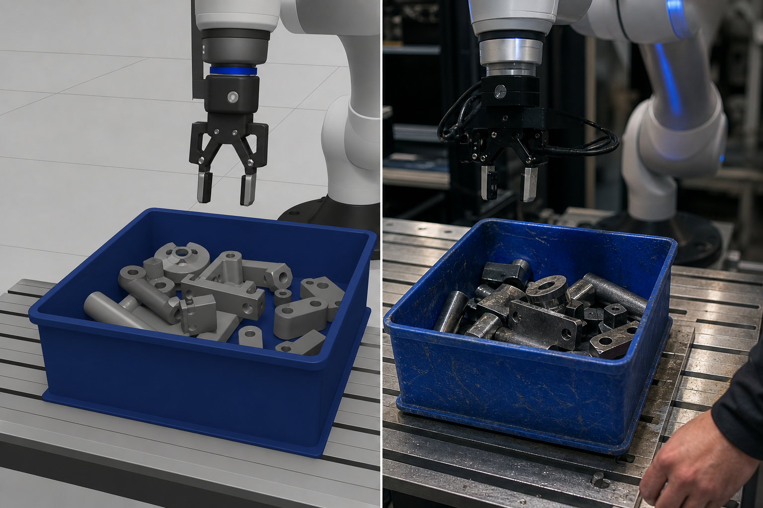
Vendor content tends to highlight successful deployments while academic sources stress ongoing challenges in robustness and sample efficiency. The honest position: domain randomization plus continual learning narrows the sim-to-real domain gap from catastrophic to manageable. It does not eliminate it. Plan for iterative retraining as a permanent line item, not a one-time project. Every long-lived sim-to-real deployment we have seen treats retraining like calibration — scheduled, instrumented, and budgeted.

Pre-Deployment Validation Checklist for Vision-Enabled Robots

Treat this as the gate before any vision-enabled robot leaves the lab. Each item is a fail-stop — if you cannot answer it with measured data, not estimates, the robot is not ready. Closed-loop control runs at 10–100 Hz, which sets the bar for every latency measurement below, as the UT Austin CS391R lectures lay out explicitly.

1. Vision inference latency measured on the actual edge hardware. Not on the development workstation. Include image capture, preprocessing (resize, normalize), inference, and post-processing in the measurement. If your control loop runs at 100 Hz (10 ms period), vision must either complete in under 10 ms or run asynchronously with motion prediction. The arXiv pragmatic guide is direct about this: synchronous edge inference that misses the cycle period creates instability that no model accuracy improvement can fix.
2. Real-hardware accuracy benchmarked at ≥80% on a held-out test set. Run at least 100 frames captured from the actual deployment environment, not from your training distribution. Log confidence scores alongside ground truth. If accuracy is below 80%, the failure mode is almost always domain gap — retrain with harder sim variants before shipping. The Robotics Perception and Control survey reports this threshold as the practical floor below which downstream control becomes unreliable.
3. Fallback behavior defined and tested for low-confidence predictions. What does the robot do when the detector returns 0.4 confidence? Options: pause and request human review, retry with a different viewpoint, abort the task. The fallback path must be tested end-to-end and must not violate safety constraints. Vision alone is fragile and needs explicit failure handling — the CS391R material is unambiguous on this point. A robot that fails loudly is safer than one that fails confidently.
4. Model quantized and optimized for the target edge stack. TensorRT for Jetson, ONNX Runtime where portable. Verify the quantized model still meets accuracy thresholds — INT8 quantization can drop accuracy 1–3 points, and that drop has to come out of your safety margin, not your performance margin. Verify thermal performance: run the vision workload at full duty cycle for 30+ minutes and confirm no thermal throttling. A model that hits target latency for the first minute and degrades after ten is a model that will fail acceptance testing.
5. Camera calibration completed and stored with the model. Intrinsics (focal length, principal point, distortion coefficients) calibrated per camera. If you are using multiple cameras, extrinsic calibration (relative poses) verified. Vision output and robot proprioception timestamps synchronized — race conditions between perception and control are a leading source of intermittent failures, per the Vision for Robotics notes. Calibration drift is also real; budget for periodic re-calibration.
6. Production telemetry pipeline live before first deployment. Log every inference: latency, confidence, predicted class, and where possible the downstream outcome (grasp success or failure). Set accuracy-drift alerts. Without telemetry, model degradation is invisible until it produces a visible incident. This is also the data feedstock for the next training cycle — the Voxel51 talk walks through how production telemetry becomes the annotation source for robot-supervised learning. If you ship without telemetry, you are shipping blind.

A robot that passes all six gates may still fail in production. A robot that fails any of the six will fail in production. Use the checklist accordingly — gate it on data, not on optimism, and require sign-off before the robot leaves the lab. Computer vision in robotics stops being a research artifact at the moment this checklist becomes a hard requirement.

Five Failure Patterns That Sink Vision-Enabled Robotics Programs

Most failed vision-in-robotics programs do not fail because the team picked the wrong model. They fail because of patterns that are visible months before deployment and ignored anyway. Each pattern below has been documented in academic and practitioner sources. Each has a known mitigation. Use this as a self-audit against your current program.

• Training on synthetic data only, validating in simulation only. Why it fails: the 90%-sim, 50%-real performance drop is the most reliably reproduced finding in the literature. What to do instead: collect at least 50–100 real-hardware frames as a held-out validation set before training begins. Never ship without a real-data accuracy number. Both the arXiv pragmatic guide and the Robotics Perception and Control survey treat real-data validation as non-negotiable, and every team that skips it relearns why.
• Single-modality dependency in adversarial conditions. Why it fails: RGB collapses in low light, depth fails on reflective and transparent surfaces, LiDAR misreads glass. Any of these conditions exists somewhere in a real deployment, and the modality that handles them well in your demo is usually the one that fails in production. What to do instead: fuse RGB with depth or LiDAR for any task touching real-world variance, as Michigan Robotics recommends as standard practice for unstructured environments.
• Treating COCO-pretrained detectors as deployment-ready. Why it fails: off-the-shelf YOLO or Faster R-CNN was trained on photographs of common objects, not on your custom industrial parts. Zero-shot accuracy on domain-specific tasks is consistently disappointing — the Vision for Robotics notes and CS391R material both flag this as a recurring trap for teams new to robotics vision. What to do instead: fine-tune on at least 20–50 task-specific examples. Even modest fine-tuning produces accuracy improvements that foundation models cannot deliver from generic pretraining alone.
• Profiling latency after the model is trained, not before. Why it fails: a 250 ms transformer feels acceptable in isolation, then the control loop budget is 10 ms and the architecture has to be re-selected. Two months of training, gone. What to do instead: define the latency budget on day one, profile candidate architectures on the target edge hardware before committing to training runs. The arXiv pragmatic guide treats early profiling as the cheapest decision a team can make.
• No continuous-improvement loop after deployment. Why it fails: real-world distributions drift — new SKUs, seasonal lighting, worn surfaces — and silent accuracy decay produces visible incidents months later. What to do instead: log every prediction with confidence, flag low-confidence frames for review, and retrain on a defined cadence or when drift is detected. The Voxel51 talk describes the robot-supervised learning loop that turns this telemetry into synthetic data annotation, and it is the difference between a deployment that gets better and one that quietly gets worse.

The fast path from environment capture to deployed robot skill is not a shortcut around these patterns — it is a workflow that makes each of them harder to commit. Real captures anchor sim. Domain randomization closes the deployment gap. Edge-target profiling locks the architecture early. Telemetry feeds the next training cycle. Run that loop end-to-end and computer vision in robotics stops being the part of the project that delays the rest.